Computer Architecture Microprocessor part 1

Objectives
Upon completion of this chapter, the reader will be able to:

1. Understand the design choices that define computer architecture.
2. Describe the different types of operations typically supported.
3. Describe common operand types and addressing modes.
4. Understand different methods for encoding data and instructions.
5. Explain control flow instructions and their types.
6. Be aware of the operation of virtual memory and its advantages.
7. Understand the difference between CISC, RISC, and VLIW architectures.
8. Understand the need for architectural extensions.

Intro

In 1964, IBM produced a series of computers beginning with the IBMThese computers were noteworthy because they all supported the
same instructions encoded in the same way; they shared a common
computer architecture. The IBM 360 and its successors were a critical
development because they allowed new computers to take advantage of
the already existing software base written for older computers. With the

advance of the microprocessor, the processor now determines the archi-
tecture of a computer.
Every microprocessor is designed to support a finite number of specific
instructions. These instructions must be encoded as binary numbers to
be read by the processor. This list of instructions, their behavior, and their
encoding define the processors’ architecture. All any processor can do is
run programs, but any program it runs must first be converted to the
instructions and encoding specific to that processor architecture. If two
processors share the same architecture, any program written for one
will run on the other and vice versa. Some example architectures and the
processors that support them are shown in Table 4-1.
The VAX architecture was introduced by Digital Equipment Corporation
(DEC) in 1977 and was so popular that new machines were still being sold
through 1999. Although no longer being supported, the VAX architecture
remains perhaps the most thoroughly studied computer architecture ever
created.
The most common desktop PC architecture is often called simply x86
after the numbering of the early Intel processors, which first defined this
architecture. This is the oldest computer architecture for which new proces-
sors are still being designed. Intel, AMD, and others carefully design new
processors to be compatible with all the software written for this archi-
tecture. Companies also often add new instructions while still supporting
all the old instructions. These architectural extensions mean that the new
processors are not identical in architecture but are backward compatible.
Programs written for older processors will run on the newer implemen-
tations, but the reverse may not be true. Intel’s Multi-Media Extension
(MMX TM ) and AMD’s 3DNow! TM are examples of “x86” architectural exten-
sions. Older programs still run on processors supporting these extensions,
but new software is required to take advantage of the new instructions.
In the early 1980s, research began into improving the performance of
microprocessors by simplifying their architectures. Early implementa-
tion efforts were led at IBM by John Cocke, at Stanford by John
Hennessy, and at Berkeley by Dave Patterson. These three teams pro-
duced the IBM 801, MIPS, and RISC-I processors. None of these were

ever sold commercially, but they inspired a new wave of architectures
referred to by the name of the Berkeley project as Reduce Instruction
Set Computers (RISC).
Sun (with direct help from Patterson) created Scalable Processor
Architecture (SPARC ® ), and Hewlett Packard created the Precision
Architecture RISC (PA-RISC). IBM created the POWER TM architecture,
which was later slightly modified to become the PowerPC architecture
now used in Macintosh computers. The fundamental difference between
Macintosh and PC software is that programs written for the Macintosh
are written in the PowerPC architecture and PC programs are written
in the x86 architecture. SPARC, PA-RISC, and PowerPC are all con-
sidered RISC architectures. Computer architects still debate their merits
compared to earlier architectures like VAX and x86, which are called
Complex Instruction Set Computers (CISC) in comparison.
Java is a high-level programming language created by Sun in 1995.
To make it easier to run programs written in Java on any computer, Sun
defined the Java Virtual Machine (JVM) architecture. This was a vir-
tual architecture because there was not any processor that actually
could run JVM code directly. However, translating Java code that had
already been compiled for a “virtual” processor was far simpler and
faster than translating directly from a high-level programming lan-
guage like Java. This allows JVM code to be used by Web sites accessed
by machines with many different architectures, as long as each machine
has its own translation program. Sun created the first physical imple-
mentation of a JVM processor in 1997.
In 2001, Intel began shipping the Itanium processor, which supported
a new architecture called Explicitly Parallel Instruction Computing
(EPIC). This architecture was designed to allow software to make more
performance optimizations and to use 64-bit addresses to allow access
to more memory. Since then, both AMD and Intel have added architectural
extensions to their x86 processors to support 64-bit memory addressing.
It is not really possible to compare the performance of different archi-
tectures independent of their implementations. The Pentium ® and
Pentium 4 processors support the same architecture, but have dramat-
ically different performance. Ultimately processor microarchitecture
and fabrication technologies will have the largest impact on perform-
ance, but the architecture can make it easier or harder to achieve high
performance for different applications. In creating a new architecture
or adding an extension to an existing architecture, designers must bal-
ance the impact to software and hardware. As a bridge from software
to hardware, a good architecture will allow efficient bug-free creation
of software while also being easily implemented in high-performance
hardware. In the end, because software applications and hardware
implementations are always changing, there is no “perfect” architecture.

Instructions

Today almost all software is written in “high-level” programming lan-
guages. Computer languages such as C, Perl, and HTML were specifi-
cally created to make software more readable and to make it independent
of a particular computer architecture. High-level languages allow the
program to concisely specify relatively complicated operations. A typical
instruction might look like:

To perform the same operation in instructions specific to a particular
processor might take several instructions.

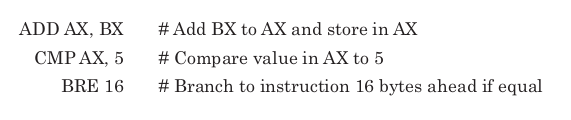
These are assembly language instructions, which are specific to a par-
ticular computer architecture. Of course, even assembly language instruc-
tions are just human readable mnemonics for the binary encoding of
instructions actually understood by the processor. The encoded binary
instructions are called machine language and are the only instructions
a processor can execute. Before any program is run on a real processor,
it must be translated into machine language. The programs that perform
this translation for high-level languages are called compilers. Translation
programs for assembly language are called assemblers. The only differ-
ence is that most assembly language instructions will be converted to a
single machine language instruction while most high-level instructions
will require multiple machine language instructions.
Software for the very first computers was written all in assembly and
was unique to each computer architecture. Today almost all programming
is done in high-level languages, but for the sake of performance small
parts of some programs are still written in assembly. Ideally, any program
written in a high-level language could be compiled to run on any proces-
sor, but the use of even small bits of architecture specific code make con-
version from one architecture to another a much more difficult task.
Although architectures may define hundreds of different instructions,
most processors spend the vast majority of their time executing only a
handful of basic instructions. Table 4-2 shows the most common types of 1
operations for the x86 architecture for the five SPECint92 benchmarks

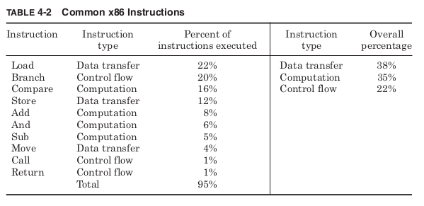
Table 4-2 shows that for programs that are considered important
measures of performance, the 10 most common instructions make up 95
percent of the total instructions executed. The performance of any imple-
mentation is determined largely by how these instructions are executed.

Computation instructions

Computational instructions create new results from operations on data
values. Any practical architecture is likely to provide the basic arithmetic
and logical operations shown in Table 4-3.
A compare instruction tests whether a particular value or pair of
values meets any of the defined conditions. Logical operations typically
treat each bit of each operand as a separate boolean value. Instructions
to shift all the bits of an operand or reverse the order of bytes make it
easier to encode multiple booleans into a single operand.
The actual operations defined by different architectures do not vary
that much. What makes different architectures most distinct from one

another is not the operations they allow, but the way in which instruc-
tions specify the inputs and outputs of their instructions. Input and
output operands are implicit or explicit. An implicit destination means
that a particular type of operation will always write its result to the same
place. Implicit operands are usually the top of the stack or a special accu-
mulator register. An explicit destination includes the intended desti-
nation as part of the instruction. Explicit operands are general-purpose
registers or memory locations. Based on the type of destination operand
supported, architectures can be classified into four basic types: stack,
accumulator, register, or memory. Table 4-4 shows how these differ-
ent architectures would implement the adding of two values stored in
memory and writing the result back to memory.
Instead of registers, the architecture can define a “stack” of stored
values. The stack is a first-in last-out queue where values are added to
the top of the stack with a push instruction and removed from the top with
a pop instruction. The concept of a stack is useful when passing many
pieces of data from one part of a program to another. Instead of having
to specify multiple different registers holding all the values, the data is
all passed on the stack. The calling subroutine pushes as many values as
needed onto the stack, and the procedure being called pops, the appro-
priate number of times to retrieve all the data. Although it would be pos-
sible to create an architecture with only load and store instructions or with
only push and pop instructions, most architectures allow for both.
A stack architecture uses the stack as an implicit source and desti-
nation. First the values A and B, which are stored in memory, are pushed
on the stack. Then the Add instruction removes the top two values on
the stack, adds them together, and pushes the result back on the stack.
The pop instruction then places this value into memory. The stack archi-
tecture Add instruction does not need to specify any operands at all
since all sources come from the stack and all results go to the stack. The
Java Virtual Machine (JVM) is a stack architecture.
An accumulator architecture uses a special register as an implicit
destination operand. In this example, it starts by loading value A into
the accumulator. Then the Add instruction reads value B from memory
and adds it to the accumulator, storing the result back in the accumu-
lator. A store instruction then writes the result out to memory.

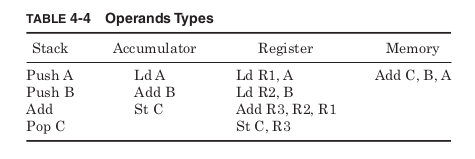
Register architectures allow the destination operand to be explicitly
specified as one of number of general-purpose registers. To perform the
example operation, first two load instructions place the values A and B
in two general-purpose registers. The Add instruction reads both these
registers and writes the results to a third. The store instruction then
writes the result to memory. RISC architectures allow register desti-
nations only for computations.
Memory architectures allow memory addresses to be given as desti-
nation operands. In this type of architecture, a single instruction might
specify the addresses of both the input operands and the address where
the result is to be stored. What might take several separate instructions
in the other architectures is accomplished in one. The x86 architecture
supports memory destinations for computations.
Many early computers were based upon stack or accumulator archi-
tectures. By using implicit operands they allow instructions to be coded
in very few bits. This was important for early computers with extremely
limited memory capacity. These early computers also executed only one
instruction at a time. However, as increased transistor budgets allowed
multiple instructions to be executed in parallel, stack and accumulator
architectures were at a disadvantage. More recent architectures have
all used register or memory destinations. The JVM architecture is an
exception to this rule, but because it was not originally intended to be
implemented in silicon, small code size and ease of translation were
deemed far more important than the possible impact on performance.
The results of one computation are commonly used as a source for
another computation, so typically the first source operand of a compu-
tation will be the same as the destination type. It wouldn’t make sense
to only support computations that write to registers if a register could
not be an input to a computation. For two source computations, the
other source could be of the same or a different type than the destina-
tion. One source could also be an immediate value, a constant encoded
as part of the instruction. For register and memory architectures, this
leads to six types of instructions. Table 4-5 shows which architectures
discussed so far provide support for which types.

The VAX architecture is the most complex, supporting all these pos-
sible combinations of source and destination types. The RISC architec-
tures are the simplest, allowing only register destinations for computations
and only immediate or register sources. The x86 architecture allows one
of the sources to be of any type but does not allow both sources to be
memory locations. Like most modern architectures, the examples in
Table 4-5 fall into three basic types shown in Table 4-6.
RISC architectures are pure register architectures, which allow reg-
ister and immediate arguments only for computations. They are also
called load/store architectures because all the movement of data to and
from memory must be accomplished with separate load and store
instructions. Register/memory architectures allow some memory
operands but do not allow all the operands to be memory locations. Pure
memory architectures support all operands being memory locations as
well as registers or immediates.
The time it takes to execute any program is the number of instruc-
tions executed times the average time per instruction. Pure register
architectures try to reduce execution time by reducing the time per
instruction. Their very simple instructions are executed quickly and
efficiently, but more of them are necessary to execute a program. Pure
memory architectures try to use the minimum number of instructions,
at the cost of increased time per instruction.
Comparing the dynamic instruction count of different architectures to an
imaginary ideal high-level language execution, Jerome Huck found pure
register architectures executing almost twice as many instructions as a pure
memory architecture implementation of the same program (Table 4-7). 3
Register/memory architectures fell between these two extremes. The high-
est performance of architectures will ultimately depend upon the imple-
mentation, but pure register architectures must execute their instructions
on average twice as fast to reach the same performance.
In addition to the operand types supported, the maximum number of
operands is chosen to be two or three. Two-operand architectures use one
source operand and a second operand which acts as both a source and
the destination. Three-operand architectures allow the destination to
be distinct from both sources. The x86 architecture is a two-operand

architecture, which can provide more compact code. The RISC archi-
tectures are three-operand architectures. The VAX architecture, seek-
ing the greatest possible flexibility in instruction type, provides for both
two- and three-operand formats.
The number and type of operands supported by different instructions
will have a great effect on how these instructions can be encoded.
Allowing for different operand encoding can greatly increase the func-
tionality and complexity of a computer architecture. The resulting size
of code and complexity in decoding will have an impact on performance.

Data transfer instructions

In addition to computational instructions, any computer architecture
will have to include data transfer instructions for moving data from
one location to another. Values may be copied from main memory to the
processor or results written out to memory. Most architectures define
registers to hold temporary values rather than requiring all data to be
accessed by a memory address. Some common data transfer instructions
and their mnemonics are listed in Table 4-8.
Loads and stores move data to and from registers and main memory.
Moves transfer data from one register to another. The conditional move
only transfers data if some specific condition is met. This condition
might be that the result of a computation was 0 or not 0, positive or not
positive, or many others. It is up to the computer architect to define all
the possible conditions that can be tested. Most architectures define a
special flag register that stores these conditions. Conditional moves can

improve performance by taking the place of instructions controlling the
program flow, which are more difficult to execute in parallel with other
instructions.
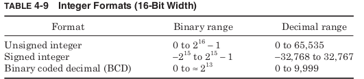
Any data being transferred will be stored as binary digits in a regis-
ter or memory location, but there are many different formats that are
used to encode a particular value in binary. The simplest formats only
support integer values. The ranges in Table 4-9 are all calculated for 16-
bit integers, but most modern architectures also support 32- and 64-bit
formats.
Unsigned format assumes every value stored is positive, and this gives
the largest positive range. Signed integers are dealt with most simply by
allowing the most significant bit to act as a sign bit, determining whether
the value is positive or negative. However, this leads to the unfortu-
nate problem of having representations for both a “positive” 0 and a
“negative” 0. As a result, signed integers are instead often stored in two’s
complement format where to reverse the sign, all the bits are negated
and 1 is added to the result. If a 0 value (represented by all 0 bits) is
negated and then has 1 added, it returns to the original zero format.
To make it easier to switch between binary and decimal representa-
tions some architectures support binary coded decimal (BCD) formats.
These treat each group of 4 bits as a single decimal digit. This is ineffi-
cient since 4 binary digits can represent 16 values rather than only 10,
but it makes conversion from binary to decimal numbers far simpler.
Storing numbers in floating-point format increases the range of
values that can be represented. Values are stored as if in scientific nota-
tion with a fraction and an exponent. IEEE standard 754 defines the for-
mats listed in Table 4-10. 4
The total number of discrete values that can be represented by inte-
ger or floating-point formats is the same, but treating some of the bits
as an exponent increases the range of values. For exponents below 1, the
possible values are closer together than an integer representation; for
exponents greater than 1, the values are farther apart. The IEEE stan-
dard reserves an exponent of all ones to represent special values like
infinity and “Not-A-Number.”

Working with floating-point numbers requires more complicated hard-
ware than integers; as a result the latency of floating-point operations
is longer than integer operations. However, the increased range of pos-
sible values is required for many graphics and scientific applications.
As a result, when quoting performance, most processors provide sepa-
rate integer and floating-point performance measurements. To improve
both integer and floating-point performance many architectures have
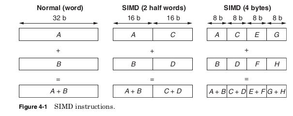
added single instruction multiple data (SIMD) operations.
SIMD instructions simultaneously perform the same computation on
multiple pieces of data (Fig. 4-1). In order to use the already defined
instruction formats, the SIMD instructions still have only two- or three-
operand instructions. However, they treat each of their operands as a
vector containing multiple pieces of data.
For example, a 64-bit register could be treated as two 32-bit integers,
four 16-bit integers, or eight 8-bit integers. Instead, the same 64-bit
register could be interpreted as two single precision floating-point num-
bers. SIMD instructions are very useful in multimedia or scientific
applications where very large amounts of data must all be processed in
the same way. The Intel MXX and AMD 3DNow! extensions both allow
operations on 64-bit vectors. Later, the Intel Streaming SIMD Extension

(SSE) and AMD 3DNow! Professional extensions provide instructions for
operating on 128-bit vectors. RISC architectures have similar extensions
including the SPARC VIS, PA-RISC MAX2, and PowerPC AltiVec.
Integer, floating-point, and vector operands show how much com-
puter architecture is affected not just by the operations allowed but by
operands allowed as well

Memory addresses

In Gulliver’s Travels by Jonathan Swift, Gulliver
finds himself in the land of Lilliput where the 6-in tall inhabitants have
been at war for years over the trivial question of how to eat a hard-boiled
egg. Should one begin by breaking open the little end or the big end? It
is unfortunate that Gulliver would find something very familiar about
one point of contention in computer architecture.
Computers universally divide their memory into groups of 8 bits called
bytes. A byte is a convenient unit because it provides just enough bits
to encode a single keyboard character. Allowing smaller units of memory
to be addressed would increase the size of memory addresses with
address bits that would be rarely used. Making the minimum address-
able unit larger could cause inefficient use of memory by forcing larger
blocks of memory to be used when a single byte would be sufficient.
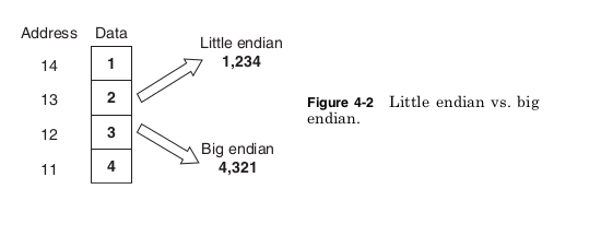
Because processors address memory by bytes but support computation
on values of more than 1 byte, a question arises: For a number of more
than 1 byte, is the byte stored at the lowest memory address the least
significant byte (the little end) or the most significant byte (the big
end)? The two sides of this debate take their names from the two fac-
tions of Lilliput: Little Endian and Big Endian. Figure 4-2 shows how
this choice leads to different results.
There are a surprising number of arguments as to why little endian
or big endian is the correct way to store data, but for most people none
of these arguments are especially convincing. As a result, each archi-
tecture has made a choice more or less at random, so that today different
computers answer this question differently. Table 4-11 shows architec-
tures that support little endian or big endian formats.
To help the sides of this debate reach mutual understanding, many
architectures support a byte swap instruction, which reverses the byte

order of a number to convert between the little endian and big endian
formats. In addition, the EPIC, PA-RISC, and PowerPC architectures
all support special modes, which cause them to read data in the oppo-
site format from their default assumption. Any new architecture will
have to pick a side or build in support for both.
Architectures must also decide whether to support unaligned memory
accesses. This would mean allowing a value of more than 1 byte to begin
at any byte in memory. Modern memory bus standards are all more
than 1-byte wide and for simplicity allow only accesses aligned on the
bus width. In other words, a 64-bit data bus will always access memory
at addresses that are multiples of 64 bits. If the architecture forces 64
bit and smaller values to be stored only at addresses that are multiples
of their width, then any value can be retrieved with a single memory
access. If the architecture allows values to start at any byte, it may
require two memory accesses to retrieve the entire value. Later accesses
of misaligned data from the cache may require multiple cache accesses.
Forcing aligned addresses improves performance, but by restricting
where values can be stored, the use of memory is made less efficient.
Given an address, the choice of little endian or big endian will deter-
mine how the data in memory is loaded. This still leaves the question
of how the address itself is generated. For any instruction that allows
a memory operand, it must be decided how the address for that memory
location will be specified. Table 4-12 shows examples of different address-
ing modes.
The simplest possible addressing is absolute mode where the memory
address is encoded as a constant in the instruction. Register indirect
addressing provides the number of a register that contains the address.
This allows the address to be computed at run time, as would be the case

for dynamically allocated variables. Displacement mode calculates the
address as the sum of a constant and a register value. Some architec-
tures allow the register value to be multiplied by a size factor. This
mode is useful for accessing arrays. The constant value can contain the
base address of the array while the registers hold the index. The size factor
allows the array index to be multiplied by the data size of the array
elements. An array of 32-bit integers will need to multiply the index
by 4 to reach the proper address because each array element contains
4 bytes.
The indexed mode is the same as the displacement mode except the
base address is held in a register rather than being a constant. The
scaled address mode sums a constant and two registers to form an
address. This could be used to access a two-dimensional array. Some
architectures also support auto increment or decrement modes where
the register being used as an index is automatically updated after the
memory access. This supports serially accessing each element of an
array. Finally, the memory indirect mode specifies a register that con-
tains the address of a memory location that contains the desired address.
This could be used to implement a memory pointer variable where the
variable itself contains a memory address.
In theory, an architecture could function supporting only register
indirect mode. However, this would require computation instructions to
form each address in a register before any memory location could be
accessed. Supporting additional addressing modes can greatly reduce the
total number of instructions required and can limit the number of reg-
isters that are used in creating addresses. Allowing a constant or a con-
stant added to a register to be used as an address is ideal for static
variables allocated during compilation. Therefore, most architectures
support at least the first three address modes listed in Table 4-12. RISC
architectures typically support only these three modes.
The more complicated modes further simplify coding but make some
memory accesses much more complex than others. Memory indirect
mode in particular requires two memory accesses for a single memory
operand. The first access retrieves the address, and the second gets the
data. VAX is one of the only architectures to support all the addressing
modes shown in Table 4-12. The x86 architecture supports all these
modes except for memory indirect. In addition to addressing modes,
modern architectures also support an additional translation of memory
addresses to be controlled by the operating system. This is called virtual
memory.

Types of memory addresses

Physical addresses

A digital computer’s main memory consists of many memory locations. Each memory location has a physical address which is a code. The CPU (or other device) can use the code to access the corresponding memory location. Generally only system software, i.e. the BIOS, operating systems, and some specialized utility programs (e.g., memory testers), address physical memory using machine code operands or processor registers, instructing the CPU to direct a hardware device, called the memory controller, to use the memory bus or system bus, or separate control, address and data busses, to execute the program’s commands. The memory controllers’ bus consists of a number of parallel lines, each represented by a binary digit (bit). The width of the bus, and thus the number of addressable storage units, and the number of bits in each unit, varies among computers.

Logical addresses

A computer program uses memory addresses to execute machine code, and to store and retrieve data. In early computers logical and physical addresses corresponded, but since the introduction of virtual memory most application programs do not have a knowledge of physical addresses. Rather, they address logical addresses, or virtual addresses, using the computer’s memory management unit and operating system memory mapping

Unit of address resolution

Most modern computers are byte-addressable. Each address identifies a single byte (eight bits) of storage. Data larger than a single byte may be stored in a sequence of consecutive addresses. There exist word-addressable computers, where the minimal addressable storage unit is exactly the processor’s word. For example, the Data General Nova minicomputer, and the Texas Instruments TMS9900 and National Semiconductor IMP-16 microcomputers used 16 bit words, and there were many 36-bit mainframe computers (e.g., PDP-10) which used 18-bit word addressing, not byte addressing, giving an address space of 2¹⁸ 36-bit words, approximately 1 megabyte of storage. The efficiency of addressing of memory depends on the bit size of the bus used for addresses – the more bits used, the more addresses are available to the computer. For example, an 8-bit-byte-addressable machine with a 20-bit address bus (e.g. Intel 8086) can address 2²⁰ (1,048,576) memory locations, or one MiB of memory, while a 32-bit bus (e.g. Intel 80386) addresses 2³² (4,294,967,296) locations, or a 4 GiB address space. In contrast, a 36-bit word-addressable machine with an 18-bit address bus addresses only 2¹⁸ (262,144) 36-bit locations (9,437,184 bits), equivalent to 1,179,648 8-bit bytes, or 1152 KB, or 1.125 MiB—slightly more than the 8086.

Some older computers (decimal computers), were decimal digit-addressable. For example, each address in the IBM 1620’s magnetic-core memory identified a single six bit binary-coded decimal digit, consisting of a parity bit, flag bit and four numerical bits. The 1620 used 5-digit decimal addresses, so in theory the highest possible address was 99,999. In practice, the CPU supported 20,000 memory locations, and up to two optional external memory units could be added, each supporting 20,000 addresses, for a total of 60,000 (00000–59999).

Virtual memory

. Early architectures allowed each program to calculate
its own memory addresses and to access memory directly using those
addresses. Each program assumed that its instructions and data would

always be located in the exact same addresses every time it ran. This
created problems when running the same program on computers with
varying amounts of memory. A program compiled assuming a certain
amount of memory might try to access more memory than the user’s
computer had. If instead, the program had been compiled assuming a
very small amount of memory, it would be unable to make use of extra
memory when running on machines that did have it.
Even more problems occurred when trying to run more than one pro-
gram simultaneously. Two different programs might both be compiled
to use the same memory addresses. When running together they could
end up overwriting each other’s data or instructions. The data from one
program read as instructions by another could cause the processor to do
almost anything. If the operating system were one of the programs over-
written, then the entire computer might lock up.
Virtual memory fixes these problems by translating each address
before memory is accessed. The address generated by the program using
the available addressing modes is called the virtual address. Before
each memory access the virtual address is translated to a physical
address. The translation is controlled by the operating system using a
lookup table stored in memory.
The lookup table needed for translations would become unmanageable
if any virtual address could be assigned any physical address. Instead,
some of the least significant virtual address bits are left untranslated.
These bits are the page offset and determine the size of a memory page.
The remaining virtual address bits form the virtual page number and
are used as an index into the lookup table to find the physical page
number. The physical page number is combined with the page offset to
make up the physical address.
The translation scheme shown in Fig. 4-3 allows every program to
assume that it will always use the exact same memory addresses, it is
the only program in memory, and the total memory size is the maximum
amount allowed by the virtual address size. The operating system deter-
mines where each virtual page will be located in physical memory. Two
programs using the same virtual address will have their addresses

translated to different physical addresses, preventing any interference.
Virtual memory cannot prevent programs from failing or having bugs,
but it can prevent these errors from causing problems in other programs.
Programs can assume more virtual memory than there is physical
memory available because not all the virtual pages need be present in
physical memory at the same time. If a program attempts to access a
virtual page not currently in memory, this is called a page fault. The pro-
gram is interrupted and the operating system moves the needed page
into memory and possibly moves another page back to the hard drive.
Once this is accomplished the original program continues from where
it was interrupted.
This slight of hand prevents the program from needing to know the
amount of memory really available. The hard drive latency is huge com-
pared to main memory, so there will be a performance impact on pro-
grams that try to use much more memory than the system really has,
but these programs will be able to run. Perhaps even more important,
programs will immediately be able to make use of new memory installed
in the system without needing to be recompiled.
The architecture defines the size of the virtual address, virtual page
number, and page offset. This determines the size of a page as well as
the maximum number of virtual pages. Any program compiled for this
architecture cannot make use of more memory than allowed by the vir-
tual address size. A large virtual address makes very large programs pos-
sible, but it also requires the processor and operating system to support
these large addresses. This is inefficient if most of the virtual address
bits are never used. As a result, each architecture chooses a virtual
address size that seems generous but not unreasonable at the time.
As Moore’s law allows the cost of memory per bit to steadily drop and
the speed of processors to steadily increase, the size of programs con-
tinues to grow. Given enough time any architecture begins to feel con-
strained by its virtual address size. A 32-bit address selects one of 2 32
bytes for a total of 4 GB of address space. When the first 32-bit proces-
sors were designed, 4 GB seemed an almost inconceivably large amount,
but today some high-performance servers already have more than 4 GB
of memory storage. As a result, the x86 architecture was extended in
2004 to add support for 64-bit addresses. A 64-bit address selects one
of 2 64 bytes, an address space 4 billion times larger than the 32-bit
address space. This will hopefully be sufficient for some years to come.
The processor, chipset, and motherboard implementation determine
the maximum physical address size. It can be larger or smaller than the
virtual address size. A physical address larger than the virtual address
means a computer system could have more physical memory than any
one program could access. This could still be useful for running multi-
ple programs simultaneously. The Pentium III supported 32-bit virtual

addresses, limiting each program to 4 GB, but it used 36-bit physical
addresses, allowing systems to use up to 64 GB of physical memory.
A physical address smaller than the virtual address simply means a
program cannot have all of its virtual pages in memory at the same time.
The EPIC architecture supports 64-bit virtual addresses, but only 50-
bit physical addresses. 5 Luckily the physical address size can be
increased from one implementation to the next while maintaining soft-
ware compatibility. Increasing virtual addresses requires recompiling
or rewriting programs if they are to make use of the larger address
space. The operating system must support both the virtual and physi-
cal address sizes, since it will determine the locations of the pages and
the permissions for accessing them.
Virtual memory is one of the most important innovations in computer
architecture. Standard desktops today commonly run dozens of programs
simultaneously; this would not be possible without virtual memory.
However, virtual memory makes very specific requirements upon the
processor. Registers as well as functional units used in computing
addresses must be able to support the virtual address size. In the worst
case, virtual memory would require two memory accesses for each memory
operand. The first would be required to read the translation from the
virtual memory lookup table and the second to access the correct physi-
cal address. To prevent this, all processors supporting virtual memory
include a cache of the most recently accessed virtual pages and their
physical page translations. This cache is called the translation lookaside
buffer (TLB) and provides translations without having to access main
memory. Only on a TLB miss, when a needed translation is not found, is
an extra memory access required. The operating system manages virtual
memory, but it is processor support that makes it practical.

Control flow instructions

Control flow instructions affect which instructions will be executed next.
They allow the linear flow of the program to be altered. Some common
control flow instructions are shown in Table 4-13.

Unconditional jumps always direct execution to a new point in the pro-
gram. Conditional jumps, also called branches, redirect or not based on
defined conditions. The same subroutines may be needed by many dif-
ferent parts of a program. To make it easy to transfer control and then
later resume execution at the same point, most architectures define call
and return instructions. A call instruction saves temporary values and
the instruction pointer (IP), which points to next instruction address,
before transferring control. The return instruction uses this informa-
tion to continue execution at the instruction after the call, with the same
architectural state. When requesting services of the operating system,
the program needs to transfer control to a subroutine that is part of the
operating system. An interrupt instruction allows this without requiring
the program to be aware of the location of the needed subroutine.
The distribution of control flow instructions measured on the SpecInt
2000 and SpecFP2000 benchmarks for the DEC Alpha architecture is
shown in Table 4-14. 6 Branches are by far the most common control flow
instruction and therefore the most important for performance.
The performance of a branch is affected by how it determines whether
it will be taken or not. Branches must have a way of explicitly or implic-
itly specifying what value is to be tested in order to decide the outcome
of the branch. The most common methods of evaluating branch condi-
tions are shown in Table 4-15.
Many architectures provide an implicit condition code register that con-
tains flags specifying important information about the most recently
calculated result. Typical flags would show whether the results were
positive or negative, zero, an overflow, or other conditions. By having all
computation instructions set the condition codes based on their result,
the comparison needed for a branch is often performed automatically. If
needed, an explicit compare instruction is used to set the condition codes
based on the comparison. The disadvantage of condition codes is they
make reordering of instructions for better performance more difficult
because every branch now depends upon the value of the condition codes.
Allowing branches to explicitly specify a condition register makes
reordering easier since different branches test different registers.

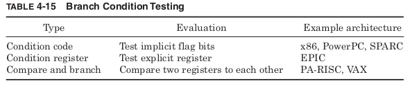
However, this approach does require more registers. Some architectures
provide a combined compare and branch instruction that performs the
comparison and switches control flow all in one instruction. This eliminates
the need for either condition codes or using condition registers but makes
the execution of a single branch instruction more complex.
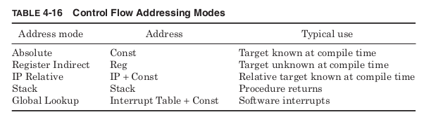
All control flow instructions must also have a way to specify the
address of the target instruction to which control is being transferred.
The common methods are listed in Table 4-16.
Absolute mode includes the target address in the control flow instruc-
tion as a constant. This works well for destination instructions with a
known address during compilation. If the target address is not known
during compilation, register indirect mode allows it to be written to a
register at run time.
The most common control flow addressing mode is IP relative address-
ing. The vast majority of control flow instructions have targets that are
very close to themselves. It is far more common to jump over a few
dozen instructions than millions. As a result, the typical size of the con-
stant needed to specify the target address is dramatically reduced if it
represents only the distance from branch to target. In IP relative
addressing, the constant is added to the current instruction pointer to
generate the target address.
Return instructions commonly make use of stack addressing, assum-
ing that the call instruction has placed the target address on the stack.
This way the same procedure can be called from many different locations
within a program and always return to the appropriate point.
Finally, software interrupt instructions typically specify a constant
that is used as an index into a global table of target addresses stored in

memory. These interrupt instructions are used to access procedures
within other applications such as the operating system. Requests to
access hardware are handled in this way without the calling program
needing any details about the type of hardware being used or even the
exact location of the handler program that will access the hardware. The
operating system maintains a global table of pointers to these various
handlers. Different handlers are loaded by changing the target addresses
in this global table.
There are three types of control flow changes that typically use global
lookup to determine their target address: software interrupts, hard-
ware interrupts, and exceptions. Software interrupts are caused by the
program executing an interrupt instruction. A software interrupt differs
from a call instruction only in how the target address is specified.
Hardware interrupts are caused by events external to the processor.
These might be a key on the keyboard being pressed, a USB device
being plugged in, a timer reaching a certain value, or many others. An
architecture cannot define all the possible hardware causes of inter-
rupts, but it must give some thought as to how they will be handled. By
using the same mechanism as software interrupts, these external events
are handled by the appropriate procedure before returning control to the
program that was running when they occurred.
Exceptions are control flow events triggered by noncontrol flow
instructions. When a divide instruction attempts to divide by 0, it is
useful to have this trigger a call to a specific procedure to deal with this
exceptional event. It makes sense that the target address for this pro-
cedure should be stored in a global table, since exceptions allow any
instruction to alter the control flow. An add that produced an overflow, a
load that caused a memory protection violation, or a push that overflowed
the stack could all trigger a change in the program flow. Exceptions are
classified by what happens after the exception procedure completes
(Table 4-17).
Fault exceptions are caused by recoverable events and return to retry
the same instruction that caused the exception. An example would be a
push instruction executed when the stack had already used all of its
available memory space. An exception handler might allocate more
memory space before allowing the push to successfully execute.

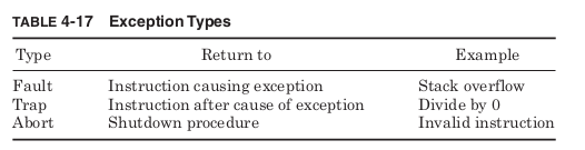
Trap exceptions are caused by events that cannot be easily fixed but
do not prevent continued execution. They return to the next instruction
after the cause of the exception. A trap handler for a divide by 0 might
print a warning message or set a variable to be checked later, but there
is no sense in retrying the divide. Abort exceptions occur when the exe-
cution can no longer continue. Attempting to execute invalid instruc-
tions, for example, would indicate that something had gone very wrong
with the program and make the correct next action unclear. An excep-
tion handler could gather information about what had gone wrong before
shutting down the program.