by Dr. Jaydeep T. Vagh
Discrete-time approximation
The bilinear transform is a first-order approximation of the natural logarithm function that is an exact mapping of the z-plane to the s-plane. When the Laplace transform is performed on a discrete-time signal (with each element of the discrete-time sequence attached to a correspondingly delayed unit impulse), the result is precisely the Z transform of the discrete-time sequence with the substitution of
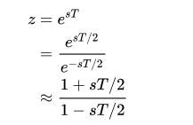
where T is the numerical integration step size of the trapezoidal rule used in the bilinear transform derivation; or, in other words, the sampling period. The above bilinear approximation can be solved for s or a similar approximation for s=(1/T)\ln(z) can be performed.
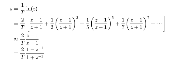

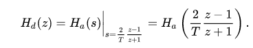
The bilinear transform essentially uses this first order approximation and substitutes into the continuous-time transfer function, Ha (s)

That is
Stability and minimum-phase property preserved
A continuous-time causal filter is stable if the poles of its transfer function fall in the left half of the complex s-plane. A discrete-time causal filter is stable if the poles of its transfer function fall inside the unit circle in the complex z-plane. The bilinear transform maps the left half of the complex s-plane to the interior of the unit circle in the z-plane. Thus, filters designed in the continuous-time domain that are stable are converted to filters in the discrete-time domain that preserve that stability.
Likewise, a continuous-time filter is minimum-phase if the zeros of its transfer function fall in the left half of the complex s-plane. A discrete-time filter is minimum-phase if the zeros of its transfer function fall inside the unit circle in the complex z-plane. Then the same mapping property assures that continuous-time filters that are minimum-phase are converted to discrete-time filters that preserve that property of being minimum-phase.
Example
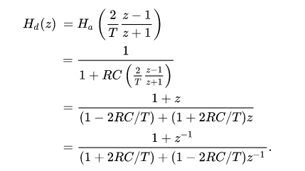
As an example take a simple low-passRC filter. This continuous-time filter has a transfer function
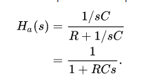

If we wish to implement this filter as a digital filter, we can apply the bilinear transform by substituting for s the formula above; after some reworking, we get the following filter representation:

The coefficients of the denominator are the ‘feed-backward’ coefficients and the coefficients of the numerator are the ‘feed-forward’ coefficients used to implement a real-time digital filter.
Transformation for a general first-order continuous-time filter
It is possible to relate the coefficients of a continuous-time, analog filter with those of a similar discrete-time digital filter created through the bilinear transform process. Transforming a general, first-order continuous-time filter with the given transfer function
using the bilinear transform (without prewarping any frequency specification) requires the substitution of
where
However, if the frequency warping compensation as described below is used in the bilinear transform, so that both analog and digital filter gain and phase agree at frequency ω 0, then
This results in a discrete-time digital filter with coefficients expressed in terms of the coefficients of the original continuous time filter:
Normally the constant term in the denominator must be normalized to 1 before deriving the corresponding difference equation. This results in
The difference equation (using the Direct Form I) is
General second-order biquad transformation
A similar process can be used for a general second-order filter with the given transfer function
This results in a discrete-time digital biquad filter with coefficients expressed in terms of the coefficients of the original continuous time filter:
Again, the constant term in the denominator is generally normalized to 1 before deriving the corresponding difference equation. This results in
The difference equation (using the Direct Form I) is
Frequency warping
o determine the frequency response of a continuous-time filter, the transfer function H a ( s ) is evaluated at s = j ω a which is on the j ω axis. Likewise, to determine the frequency response of a discrete-time filter, the transfer function H d ( z ) is evaluated at z = e j ω d T which is on the unit circle, | z | = 1 . The bilinear transform maps the j ω axis of the s-plane (of which is the domain of H a ( s ) to the unit circle of the z-plane, | z | = 1 (which is the domain of H d ( z ) , but it is not the same mapping z = e s T which also maps the j ωaxis to the unit circle. When the actual frequency of ω d is input to the discrete-time filter designed by use of the bilinear transform, then it is desired to know at what frequency, ω a, for the continuous-time filter that this ω d is mapped to.

This shows that every point on the unit circle in the discrete-time filter z-plane, z = e j ω d T is mapped to a point on the j ω j omega axis on the continuous-time filter s-plane, s = j ω a . That is, the discrete-time to continuous-time frequency mapping of the bilinear transform is

and the inverse mapping is

The discrete-time filter behaves at frequency ω d the same way that the continuous-time filter behaves at frequency ( 2 / T ) tan ( ω d T / 2 ) . Specifically, the gain and phase shift that the discrete-time filter has at frequency ω d is the same gain and phase shift that the continuous-time filter has at frequency ( 2 / T ) tan ( ω d T / 2 ) . This means that every feature, every “bump” that is visible in the frequency response of the continuous-time filter is also visible in the discrete-time filter, but at a different frequency. For low frequencies (that is, when ω d ≪ 2 / T or ω a ≪ 2 / T, then the features are mapped to a slightly different frequency; ω d ≈ ω a
One can see that the entire continuous frequency range
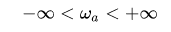
is mapped onto the fundamental frequency interval

The continuous-time filter frequency ω a = 0 corresponds to the discrete-time filter frequency ω d = 0 and the continuous-time filter frequency ω a = ± ∞ correspond to the discrete-time filter frequency ω d = ± π / T .
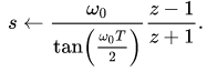
One can also see that there is a nonlinear relationship between ω a and ω d . This effect of the bilinear transform is called frequency warping. The continuous-time filter can be designed to compensate for this frequency warping by setting

for every frequency specification that the designer has control over (such as corner frequency or center frequency). This is called pre-warping the filter design.
It is possible, however, to compensate for the frequency warping by pre-warping a frequency specification ω 0(usually a resonant frequency or the frequency of the most significant feature of the frequency response) of the continuous-time system. These pre-warped specifications may then be used in the bilinear transform to obtain the desired discrete-time system. When designing a digital filter as an approximation of a continuous time filter, the frequency response (both amplitude and phase) of the digital filter can be made to match the frequency response of the continuous filter at a specified frequency ω 0, as well as matching at DC, if the following transform is substituted into the continuous filter transfer function.[2] This is a modified version of Tustin’s transform shown above
However, note that this transform becomes the original transform

The main advantage of the warping phenomenon is the absence of aliasing distortion of the frequency response characteristic, such as observed with Impulse invariance.
