by Dr. Jaydeep T. Vagh
That mathematical knowledge only parpose in Signal processing
In mathematics, the discrete Fourier transform (DFT) converts a finite sequence of equally-spaced samples of a function into a same-length sequence of equally-spaced samples of the discrete-time Fourier transform (DTFT), which is a complex-valued function of frequency. The interval at which the DTFT is sampled is the reciprocal of the duration of the input sequence. An inverse DFT is a Fourier series, using the DTFT samples as coefficients of complex sinusoids at the corresponding DTFT frequencies. It has the same sample-values as the original input sequence. The DFT is therefore said to be a frequency domain representation of the original input sequence. If the original sequence spans all the non-zero values of a function, its DTFT is continuous (and periodic), and the DFT provides discrete samples of one cycle. If the original sequence is one cycle of a periodic function, the DFT provides all the non-zero values of one DTFT cycle
The DFT is the most important discrete transform, used to perform Fourier analysis in many practical applications.[1] In digital signal processing, the function is any quantity or signal that varies over time, such as the pressure of a sound wave, a radio signal, or daily temperature readings, sampled over a finite time interval (often defined by a window function[2]). In image processing, the samples can be the values of pixels along a row or column of a raster image. The DFT is also used to efficiently solve partial differential equations, and to perform other operations such as convolutions or multiplying large integers.
Since it deals with a finite amount of data, it can be implemented in computers by numerical algorithms or even dedicated hardware. These implementations usually employ efficient fast Fourier transform (FFT) algorithms;[3] so much so that the terms “FFT” and “DFT” are often used interchangeably. Prior to its current usage, the “FFT” initialism may have also been used for the ambiguous term “finite Fourier transform”.
Definition
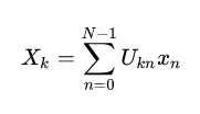
The discrete Fourier transform transforms a sequence of N complex numbers { x n } := x 0 , x 1 , … , x N − 1 into another sequence of complex numbers, { X k } := X 0 , X 1 , … , X N − 1 , which is defined by
where the last expression follows from the first one by Euler’s formula.
The transform is sometimes denoted by the symbol
Motivation
Eq.1 can also be evaluated outside the domain
and that extended sequence is N N-periodic. Accordingly, other sequences of N indices are sometimes used, such as

(if N N is even) and

which amounts to swapping the left and right halves of the result of the transform.
Eq.1 can be interpreted or derived in various ways, for example:
- It completely describes the discrete-time Fourier transform (DTFT) of an N -periodic sequence, which comprises only discrete frequency components. (Using the DTFT with periodic data)
- It can also provide uniformly spaced samples of the continuous DTFT of a finite length sequence. (Sampling the DTFT)
- It is the cross correlation of the input sequence, x n, and a complex sinusoid at frequency k/ N . Thus it acts like a matched filter for that frequency.
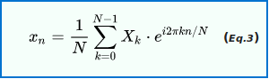
- It is the discrete analog of the formula for the coefficients of a Fourier series:

which is also NN-periodic. In the domain n ∈ [0, N − 1], this is the inverse transform of Eq.1. In this interpretation, each X is a complex number that encodes both amplitude and phase of a complex sinusoidal component ( e i 2 π k n / N )
of function x n .The sinusoid’s frequency is k cycles per N samples. Its amplitude and phase are:

where atan2 is the two-argument form of the arctan function. In polar form

here cis is the mnemonic for cos + i sin.
The normalization factor multiplying the DFT and IDFT (here 1 and 1/N) and the signs of the exponents are merely conventions, and differ in some treatments. The only requirements of these conventions are that the DFT and IDFT have opposite-sign exponents and that the product of their normalization factors be 1 / N 1/N. A normalization of 1 / N for both the DFT and IDFT, for instance, makes the transforms unitary. A discrete impulse, x n = 1 at n = 0 and 0 otherwise; might transform to X k = 1 for all k (use normalization factors 1 for DFT and 1/N for IDFT). A DC signal, X k = 1 at k = 0 and 0 otherwise; might inversely transform to x n = 1 for all n 1/N for DFT and 1 for IDFT) which is consistent with viewing DC as the mean average of the signal.
Inverse transform
The discrete Fourier transform is an invertible, linear transformation

with C denoting the set of complex numbers. This is known as Inverse Discrete Fourier Transform(IDFT). In other words, for any N > 0 N>0, an N-dimensional complex vector has a DFT and an IDFT which are in turn N N-dimensional complex vectors.
The inverse transform is given by:
Properties
Linearity
The DFT is a linear transform

then for any complex numbers a,b:
Time and frequency reversal
Reversing the time in x n to reversing the frequency Mathematically, if { x n } represents the vector x then Reversing the time in x n to reversing the frequency

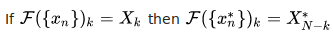
Conjugation in time
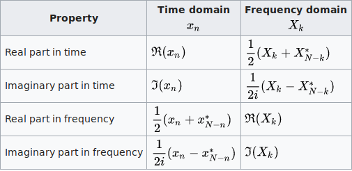
Real and imaginary part
This table shows some mathematical operations on x n in the time domain and the corresponding effects on its DFT X k in the frequency domain.
Orthogonality

where δ k k ′ is the Kronecker delta. (In the last step, the summation is trivial if k = k ′ k=k’, where it is 1+1+⋅⋅⋅=N, and otherwise is a geometric series that can be explicitly summed to obtain zero.) This orthogonality condition can be used to derive the formula for the IDFT from the definition of the DFT, and is equivalent to the unitarity property below.
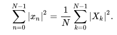
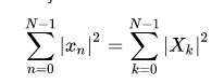
The Plancherel theorem and Parseval’s theorem
If X k the DFTs of x n respectively then the Parseval’s theorem states:

where the star denotes complex conjugation. Plancherel theorem is a special case of the Parseval’s theorem and states:
These theorems are also equivalent to the unitary condition below.
Periodicity
The periodicity can be shown directly from the definition:

Similarly, it can be shown that the IDFT formula leads to a periodic extension.
Shift theorem

Circular convolution theorem and cross-correlation theorem
The convolution theorem for the discrete-time Fourier transform indicates that a convolution of two infinite sequences can be obtained as the inverse transform of the product of the individual transforms. An important simplification occurs when the sequences are of finite length, N. In terms of the DFT and inverse DFT, it can be written as follows:

which is the convolution of the x sequence with a y sequence extended by periodic summation:

Similarly, the cross-correlation of x and y N is given by:

When either sequence contains a string of zeros, of length L L+1 of the circular convolution outputs are equivalent to values of x ∗ y . . Methods have also been developed to use this property as part of an efficient process that constructs x ∗ y with an x or y sequence potentially much longer than the practical transform size ( N N). Two such methods are called overlap-save and overlap-add.[6] The efficiency results from the fact that a direct evaluation of either summation (above) requires O ( N 2 ) ) operations for an output sequence of length N N. An indirect method, using transforms, can take advantage of the O ( N log N ) \scriptstyle O(N\log N) efficiency of the fast Fourier transform (FFT) to achieve much better performance. Furthermore, convolutions can be used to efficiently compute DFTs via Rader’s FFT algorithm and Bluestein’s FFT algorithm.
Convolution theorem duality
It can also be shown that:

Trigonometric interpolation polynomial
The trigonometric interpolation polynomial

where the coefficients Xk are given by the DFT of xn above, satisfies the interpolation property p ( n / N ) = x n for n = 0 , … , N − 1 n=0,\ldots ,N-1.
For even N, notice that the Nyquist component

is handled specially.
This interpolation is not unique: aliasing implies that one could add N to any of the complex-sinusoid frequencies (e.g. changing e − i t ) without changing the interpolation property, but giving different values in between the x n points. The choice above, however, is typical because it has two useful properties. First, it consists of sinusoids whose frequencies have the smallest possible magnitudes: the interpolation is bandlimited. Second, if the x n are real numbers, then p ( t ) p(t) is real as well.
In contrast, the most obvious trigonometric interpolation polynomial is the one in which the frequencies range from 0 to N − 1 N-1 (instead of roughly − N / 2 -N/2 to + N / 2 +N/2 as above), similar to the inverse DFT formula. This interpolation does not minimize the slope, and is not generally real-valued for real x n its use is a common mistake.
The unitary DFT
Another way of looking at the DFT is to note that in the above discussion, the DFT can be expressed as the DFT matrix, a Vandermonde matrix, introduced by Sylvester in 1867,

The inverse transform is then given by the inverse of the above matrix,
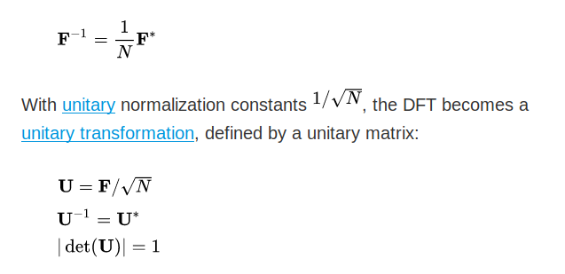
where det is the determinant function. The determinant is the product of the eigenvalues, which are always \pm 1 or \pm i as described below. In a real vector space, a unitary transformation can be thought of as simply a rigid rotation of the coordinate system, and all of the properties of a rigid rotation can be found in the unitary DFT.
The orthogonality of the DFT is now expressed as an orthonormality condition (which arises in many areas of mathematics as described in root of unity):
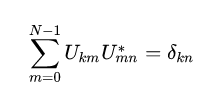
If X is defined as the unitary DFT of the vector x, then
and the Plancherel theorem is expressed as

If we view the DFT as just a coordinate transformation which simply specifies the components of a vector in a new coordinate system, then the above is just the statement that the dot product of two vectors is preserved under a unitary DFT transformation. For the special case x = y , this implies that the length of a vector is preserved as well—this is just Parseval’s theorem,
A consequence of the circular convolution theorem is that the DFT matrix F diagonalizes any circulant matrix.
Expressing the inverse DFT in terms of the DFT
A useful property of the DFT is that the inverse DFT can be easily expressed in terms of the (forward) DFT, via several well-known “tricks”. (For example, in computations, it is often convenient to only implement a fast Fourier transform corresponding to one transform direction and then to get the other transform direction from the first.)
First, we can compute the inverse DFT by reversing all but one of the inputs (Duhamel et al., 1988):

(As usual, the subscripts are interpreted modulo N; thus, for n = 0 n=0, we have x N − 0 = x 0
Second, one can also conjugate the inputs and outputs:

Third, a variant of this conjugation trick, which is sometimes preferable because it requires no modification of the data values, involves swapping real and imaginary parts (which can be done on a computer simply by modifying pointers). Define swap ( x n ) ) ) as x n with its real and imaginary parts swapped—that is, if x n = a + b i x_{n}=a+bi then swap ( x n ) is b + a i b+ai. Equivalently, swap ( x n ) \operatorname ) equals i x n ∗ . Then

That is, the inverse transform is the same as the forward transform with the real and imaginary parts swapped for both input and output, up to a normalization (Duhamel et al., 1988).
The conjugation trick can also be used to define a new transform, closely related to the DFT, that is involutory—that is, which is its own inverse. In particular T is clearly its ownThe conjugation trick can also be used to define a new transform, closely related to the DFT, that is involutory—that is, which is its own inverse. In particular
Eigenvalues and eigenvectors
The eigenvalues of the DFT matrix are simple and well-known, whereas the eigenvectors are complicated, not unique, and are the subject of ongoing research.
Consider the unitary form U defined above for the DFT of length N, where

This matrix satisfies the matrix polynomial equation:
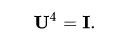
This can be seen from the inverse properties above: operating U twice gives the original data in reverse order, so operating U four times gives back the original data and is thus the identity matrix. This means that the eigenvalues λ lambda satisfy the equation:

Therefore, the eigenvalues of U \lambda is +1, −1, +i, or −i.
Since there are only four distinct eigenvalues for this N × N {\displaystyle N\times N} N\times N matrix, they have some multiplicity. The multiplicity gives the number of linearly independent eigenvectors corresponding to each eigenvalue. (There are N independent eigenvectors; a unitary matrix is never defective.)
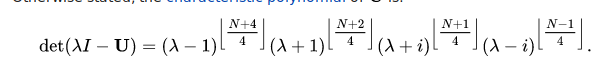
The problem of their multiplicity was solved by McClellan and Parks (1972), although it was later shown to have been equivalent to a problem solved by Gauss (Dickinson and Steiglitz, 1982). The multiplicity depends on the value of N modulo 4, and is given by the following table:

Otherwise stated, the characteristic polynomial of U is:
No simple analytical formula for general eigenvectors is known. Moreover, the eigenvectors are not unique because any linear combination of eigenvectors for the same eigenvalue is also an eigenvector for that eigenvalue. Various researchers have proposed different choices of eigenvectors, selected to satisfy useful properties like orthogonality and to have “simple” forms (e.g., McClellan and Parks, 1972; Dickinson and Steiglitz, 1982; Grünbaum, 1982; Atakishiyev and Wolf, 1997; Candan et al., 2000; Hanna et al., 2004; Gurevich and Hadani, 2008).
A straightforward approach is to discretize an eigenfunction of the continuous Fourier transform, of which the most famous is the Gaussian function. Since periodic summation of the function means discretizing its frequency spectrum and discretization means periodic summation of the spectrum, the discretized and periodically summed Gaussian function yields an eigenvector of the discrete transform:
The closed form expression for the series can be expressed by Jacobi theta functions as

Two other simple closed-form analytical eigenvectors for special DFT period N were found (Kong, 2008):
For DFT period N = 2L + 1 = 4K + 1, where K is an integer, the following is an eigenvector of DFT:

The choice of eigenvectors of the DFT matrix has become important in recent years in order to define a discrete analogue of the fractional Fourier transform—the DFT matrix can be taken to fractional powers by exponentiating the eigenvalues (e.g., Rubio and Santhanam, 2005). For the continuous Fourier transform, the natural orthogonal eigenfunctions are the Hermite functions, so various discrete analogues of these have been employed as the eigenvectors of the DFT, such as the Kravchuk polynomials (Atakishiyev and Wolf, 1997). The “best” choice of eigenvectors to define a fractional discrete Fourier transform remains an open question, however.
Uncertainty principles
Probabilistic uncertainty principle
If the random variable Xk is constrained by

then

may be considered to represent a discrete probability mass function of n, with an associated probability mass function constructed from the transformed variable,

For the case of continuous functions P ( x ) Q(k), the Heisenberg uncertainty principle states that
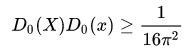
where D 0 ( X ) (x) are the variances of | X | 2 respectively, with the equality attained in the case of a suitably normalized Gaussian distribution. Although the variances may be analogously defined for the DFT, an analogous uncertainty principle is not useful, because the uncertainty will not be shift-invariant. Still, a meaningful uncertainty principle has been introduced by Massar and Spindel.
However, the Hirschman entropic uncertainty will have a useful analog for the case of the DFT. The Hirschman uncertainty principle is expressed in terms of the Shannon entropy of the two probability functions.
In the discrete case, the Shannon entropies are defined as
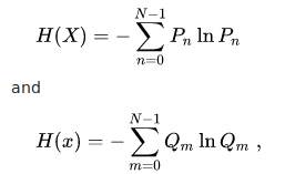
and the entropic uncertainty principle becomes

The equality is obtained for P nequal to translations and modulations of a suitably normalized Kronecker comb of period A A where A is any exact integer divisor of N. The probability mass function Q mwill then be proportional to a suitably translated Kronecker comb of period B = N / A
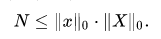
Deterministic uncertainty principle
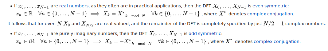
DFT of real and purely imaginary signals
Generalized DFT (shifted and non-linear phase)
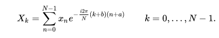
is possible to shift the transform sampling in time and/or frequency domain by some real shifts a and b, respectively. This is sometimes known as a generalized DFT (or GDFT), also called the shifted DFT or offset DFT, and has analogous properties to the ordinary DFT:
Most often, shifts of 1 / 2 (half a sample) are used. While the ordinary DFT corresponds to a periodic signal in both time and frequency domains, a = 1 / 2produces a signal that is anti-periodic in frequency domain. Such shifted transforms are most often used for symmetric data, to represent different boundary symmetries, and for real-symmetric data they correspond to different forms of the discrete cosine and sine transforms.
Another interesting choice is a = b = − ( N − 1 ) / 2 a=b=-(N-1)/2, which is called the centered DFT (or CDFT). The centered DFT has the useful property that, when N is a multiple of four, all four of its eigenvalues (see above) have equal multiplicities (Rubio and Santhanam, 2005)
The term GDFT is also used for the non-linear phase extensions of DFT. Hence, GDFT method provides a generalization for constant amplitude orthogonal block transforms including linear and non-linear phase types. GDFT is a framework to improve time and frequency domain properties of the traditional DFT, e.g. auto/cross-correlations, by the addition of the properly designed phase shaping function (non-linear, in general) to the original linear phase functions (Akansu and Agirman-Tosun, 2010).
The discrete Fourier transform can be viewed as a special case of the z-transform, evaluated on the unit circle in the complex plane; more general z-transforms correspond to complex shifts a and b above.
Multidimensional DFT
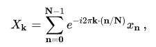
The ordinary DFT transforms a one-dimensional sequence or array x n that is a function of exactly one discrete variable n. The multidimensional DFT of a multidimensional array x n 1 , n 2 , … , n d that is a function of d discrete variables n ℓ = 0 , 1 , … , N ℓ − 1 ,d is defined by:

where ω N ℓ = exp ( − i 2 π / N ℓ ) as above and the d output indices run from k ℓ = 0 , 1 , … , N ℓ -1. This is more compactly expressed in vector notation, where we define n = ( n 1 , n 2 , … , n d ) and k = ( k 1 , k 2 , … , k d ) as d-dimensional vectors of indices from 0 to N − 1 , which we define as N − 1 = ( N 1 − 1 , N 2 − 1 , … , N d − 1 )
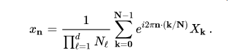
where the division n / N is defined as n / N = ( n 1 / N 1 , … , n d / N d ) to be performed element-wise, and the sum denotes the set of nested summations above.
The inverse of the multi-dimensional DFT is, analogous to the one-dimensional case, given by:
As the one-dimensional DFT expresses the input x n as a superposition of sinusoids, the multidimensional DFT expresses the input as a superposition of plane waves, or multidimensional sinusoids. The direction of oscillation in space is k / N . This decomposition is of great importance for everything from digital image processing (two-dimensional) to solving partial differential equations. The solution is broken up into plane waves.
The multidimensional DFT can be computed by the composition of a sequence of one-dimensional DFTs along each dimension. In the two-dimensional case x n 1 , n 2 independent DFTs of the rows (i.e., along n 2) are computed first to form a new array y n 1 , k 2 . Then the N 2 independent DFTs of y along the columns (along n 1 are computed to form the final result X k 1 , k 2 . Alternatively the columns can be computed first and then the rows. The order is immaterial because the nested summations above commute.
An algorithm to compute a one-dimensional DFT is thus sufficient to efficiently compute a multidimensional DFT. This approach is known as the row-column algorithm. There are also intrinsically multidimensional FFT algorithms.
The real-input multidimensional DFT
For input data x n 1 , n 2 , … , n d consisting of real numbers, the DFT outputs have a conjugate symmetry similar to the one-dimensional case above:

where the star again denotes complex conjugation and the ℓell -th subscript is again interpreted modulo N
