by Dr. Jaydeep T. Vagh
In mathematics, the discrete-time Fourier transform (DTFT) is a form of Fourier analysis that is applicable to a sequence of values.
The DTFT is often used to analyze samples of a continuous function. The term discrete-time refers to the fact that the transform operates on discrete data, often samples whose interval has units of time. From uniformly spaced samples it produces a function of frequency that is a periodic summation of the continuous Fourier transform of the original continuous function. Under certain theoretical conditions, described by the sampling theorem, the original continuous function can be recovered perfectly from the DTFT and thus from the original discrete samples. The DTFT itself is a continuous function of frequency, but discrete samples of it can be readily calculated via the discrete Fourier transform (DFT) (see Sampling the DTFT), which is by far the most common method of modern Fourier analysis.
Both transforms are invertible. The inverse DTFT is the original sampled data sequence. The inverse DFT is a periodic summation of the original sequence. The fast Fourier transform (FFT) is an algorithm for computing one cycle of the DFT, and its inverse produces one cycle of the inverse DFT.
Definition
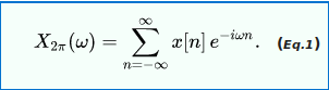
The discrete-time Fourier transform of a discrete set of real or complex numbers x[n], for all integers n, is a Fourier series, which produces a periodic function of a frequency variable. When the frequency variable, ω, has normalized units of radians/sample, the periodicity is 2π, and the Fourier series is:
The utility of this frequency domain function is rooted in the Poisson summation formula. Let X(f) be the Fourier transform of any function, x(t), whose samples at some interval T (seconds) are equal (or proportional) to the x[n] sequence, i.e. T⋅x(nT) = x[n]. Then the periodic function represented by the Fourier series is a periodic summation of X(f) in terms of frequency f in hertz (cycles/sec):
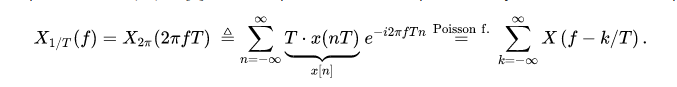
The integer k has units of cycles/sample, and 1/T is the sample-rate, fs (samples/sec). So X1/T(f) comprises exact copies of X(f) that are shifted by multiples of fs hertz and combined by addition. For sufficiently large fs the k = 0 term can be observed in the region [−fs/2, fs/2] with little or no distortion (aliasing) from the other terms. In Fig.1, the extremities of the distribution in the upper left corner are masked by aliasing in the periodic summation (lower left).
We also note that e−i2πfTn is the Fourier transform of δ(t − nT). Therefore, an alternative definition of DTFT is:

The modulated Dirac comb function is a mathematical abstraction sometimes referred to as impulse sampling.
Inverse transform
An operation that recovers the discrete data sequence from the DTFT function is called an inverse DTFT. For instance, the inverse continuous Fourier transform of both sides of Eq.3 produces the sequence in the form of a modulated Dirac comb function:
However, noting that X1/T(f) is periodic, all the necessary information is contained within any interval of length 1/T. In both Eq.1 and Eq.2, the summations over n are a Fourier series, with coefficients x[n]. The standard formulas for the Fourier coefficients are also the inverse transforms:
Periodic data
When the input data sequence x[n] is N-periodic, Eq.2 can be computationally reduced to a discrete Fourier transform (DFT), because:
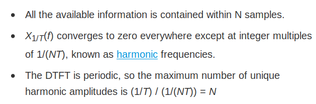
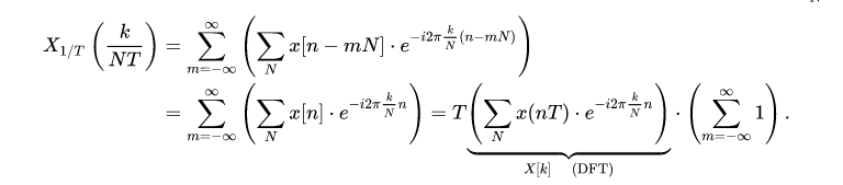
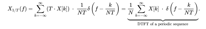
Therefore, the DTFT diverges at the harmonic frequencies, but at different frequency-dependent rates. And those rates are given by the DFT of one cycle of the x[n] sequence. In terms of a Dirac comb function, this is represented by:
Sampling the DTFT
When the DTFT is continuous, a common practice is to compute an arbitrary number of samples (N) of one cycle of the periodic function X1/T:
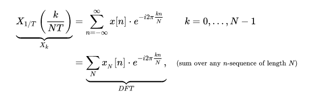
where is a periodic summation:

The N sequence is the inverse DFT. Thus, our sampling of the DTFT causes the inverse transform to become periodic. The array of |Xk|2 values is known as a periodogram, and the parameter N is called NFFT in the Matlab function of the same name.
In order to evaluate one cycle of numerically, we require a finite-length x[n] sequence. For instance, a long sequence might be truncated by a window function of length L resulting in three cases worthy of special mention. For notational simplicity, consider the x[n] values below to represent the values modified by the window function.
Case: Frequency decimation. L = N ⋅ I, for some integer I (typically 6 or 8)
A cycle of x N reduces to a summation of I blocks of length N, or circular addition. The DFT then goes by various names, such as:
- window-presum FFT
- Weight, overlap, add (WOLA)
- polyphase FFT
- polyphase filter bank
- multiple block windowing and time-aliasing.

Recall that decimation of sampled data in one domain (time or frequency) produces overlap (sometimes known as aliasing) in the other, and vice versa. Compared to an L-length DFT, the xN summation/overlap causes decimation in frequency, leaving only DTFT samples least affected by spectral leakage. That is usually a priority when implementing an FFT filter-bank (channelizer). With a conventional window function of length L, scalloping loss would be unacceptable. So multi-block windows are created using FIR filter design tools. Their frequency profile is flat at the highest point and falls off quickly at the midpoint between the remaining DTFT samples. The larger the value of parameter I, the better the potential performance.
Case: L = N+1, where N is even-valued
This case arises in the context of Window function design, out of a desire for real-valued DFT coefficients. When a symmetric sequence is associated with the indices [-M ≤ n ≤ M], known as a finite Fourier transform data window, its DTFT, a continuous function of frequency f(n) is real-valued. When the sequence is shifted into a DFT data window, [0 ≤ n ≤ 2M], the DTFT is multiplied by a complex-valued phase function: e − i2πfMBut when sampled at frequencies f=k / 2M for integer values of k he samples are all real-valued. To achieve that goal, we can perform a 2 -length DFT on a periodic summation with 1-sample of overlap. Specifically, the last sample of a data sequence is deleted and its value added to the first sample. Then a window function, shortened by 1 sample, is applied, and the DFT is performed. The shortened, even-length window function is sometimes called DFT-even. In actual practice, people commonly use DFT-even windows without overlapping the data, because the detrimental effects on spectral leakage are negligible for long sequences (typically hundreds of samples).
Convolution
The convolution theorem for sequences is:

An important special case is the circular convolution of sequences x and y defined by x N ∗ y where x N is a periodic summation. The discrete-frequency nature of DTFT{xN} “selects” only discrete values from the continuous function DTFT{y}, which results in considerable simplification of the inverse transform. As shown at Convolution theorem#Functions of discrete variable sequences:

For x and y sequences whose non-zero duration is less than or equal to N, a final simplification is:

The significance of this result is expounded at Circular convolution and Fast convolution algorithms.
Symmetry properties
When the real and imaginary parts of a complex function are decomposed into their even and odd parts, there are four components, denoted below by the subscripts RE, RO, IE, and IO. And there is a one-to-one mapping between the four components of a complex time function and the four components of its complex frequency transform
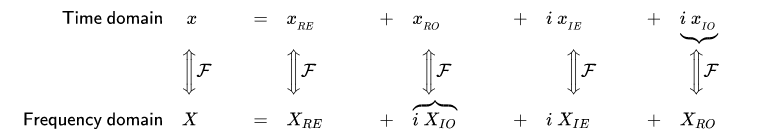
From this, various relationships are apparent, for example:

Relationship to the Z-transform
X 2 π ( ω ) is a Fourier series that can also be expressed in terms of the bilateral Z-transform. I.e.:
where the X ^ notation distinguishes the Z-transform from the Fourier transform. Therefore, we can also express a portion of the Z-transform in terms of the Fourier transform:
Note that when parameter T changes, the terms of X 2 π ( ω ) remain a constant separation 2 π apart, and their width scales up or down. The terms of X1/T(f) remain a constant width and their separation 1/T scales up or down.
Table of discrete-time Fourier transforms
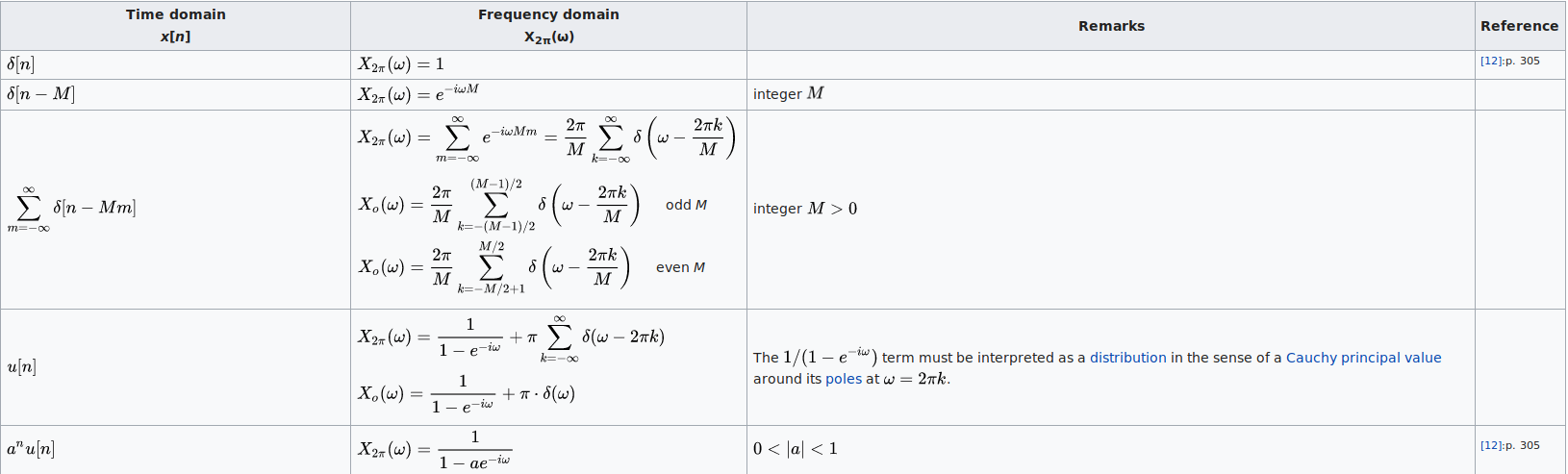
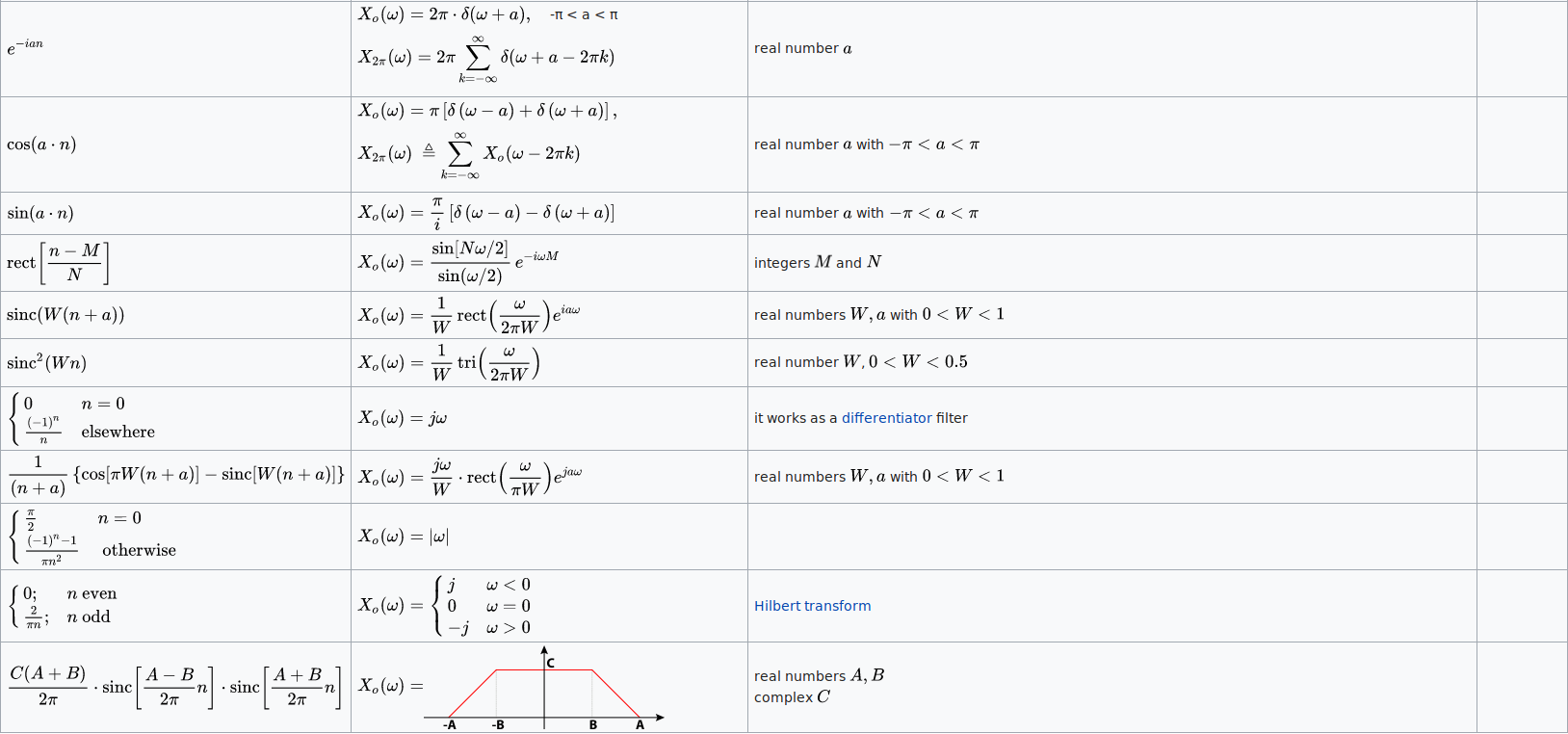
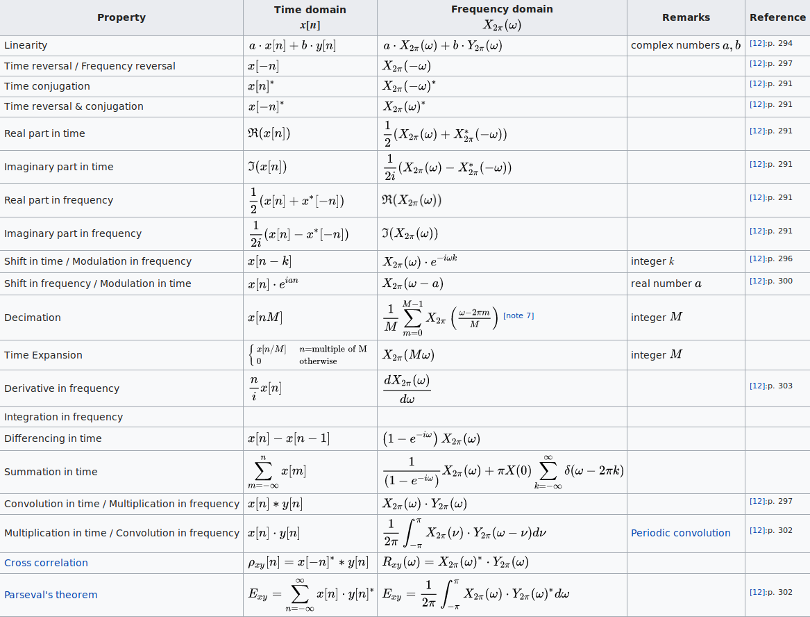
Properties
This table shows some mathematical operations in the time domain and the corresponding effects in the frequency domain.