Laplace transform

by Dr. Jaydeep T. Vagh

In mathematics, the Laplace transform is an integral transform named after its inventor Pierre-Simon Laplace (/ləˈplɑːs/). It transforms a function of a real variable t (often time) to a function of a complex variable s (complex frequency). The transform has many applications in science and engineering.

The Laplace transform is similar to the Fourier transform. While the Fourier transform of a function is a complex function of a real variable (frequency), the Laplace transform of a function is a complex function of a complex variable. Laplace transforms are usually restricted to functions of t with t ≥ 0. A consequence of this restriction is that the Laplace transform of a function is a holomorphic function of the variable s. Unlike the Fourier transform, the Laplace transform of a distribution is generally a well-behaved function. Techniques of complex variables can also be used to directly study Laplace transforms. As a holomorphic function, the Laplace transform has a power series representation. This power series expresses a function as a linear superposition of moments of the function. This perspective has applications in probability theory.

The Laplace transform is invertible on a large class of functions. The inverse Laplace transform takes a function of a complex variable s (often frequency) and yields a function of a real variable t (often time). Given a simple mathematical or functional description of an input or output to a system, the Laplace transform provides an alternative functional description that often simplifies the process of analyzing the behavior of the system, or in synthesizing a new system based on a set of specifications.[1] So, for example, Laplace transformation from the time domain to the frequency domain transforms differential equations into algebraic equations and convolution into multiplication.

Laplace wrote extensively about the use of generating functions in Essai philosophique sur les probabilités (1814) and the integral form of the Laplace transform evolved naturally as a result

History

The Laplace transform is named after mathematician and astronomer Pierre-Simon Laplace, who used a similar transform in his work on probability theory. Laplace’s use of generating functions was similar to what is now known as the z-transform and he gave little attention to the continuous variable case which was discussed by Niels Henrik Abel. The theory was further developed in the 19th and early 20th centuries by Mathias Lerch, Oliver Heaviside, and Thomas Bromwich.[7] The current widespread use of the transform (mainly in engineering) came about during and soon after World War II replacing the earlier Heaviside operational calculus. The advantages of the Laplace transform had been emphasized by Gustav Doetsch to whom the name Laplace Transform is apparently due.

The early history of methods having some similarity to Laplace transform is as follows. From 1744, Leonhard Euler investigated integrals of the form

as solutions of differential equations but did not pursue the matter very far.

Joseph Louis Lagrange was an admirer of Euler and, in his work on integrating probability density functions, investigated expressions of the form

which some modern historians have interpreted within modern Laplace transform theory

These types of integrals seem first to have attracted Laplace’s attention in 1782 where he was following in the spirit of Euler in using the integrals themselves as solutions of equations.[13] However, in 1785, Laplace took the critical step forward when, rather than just looking for a solution in the form of an integral, he started to apply the transforms in the sense that was later to become popular. He used an integral of the form

akin to a Mellin transform, to transform the whole of a difference equation, in order to look for solutions of the transformed equation. He then went on to apply the Laplace transform in the same way and started to derive some of its properties, beginning to appreciate its potential power.

Laplace also recognised that Joseph Fourier’s method of Fourier series for solving the diffusion equation could only apply to a limited region of space because those solutions were periodic. In 1809, Laplace applied his transform to find solutions that diffused indefinitely in space.

Formal definition

The Laplace transform of a function f(t), defined for all real numbers t ≥ 0, is the function F(s), which is a unilateral transform defined by

where s is a complex number frequency parameter

An alternate notation for the Laplace transform is L instead of F.

The meaning of the integral depends on types of functions of interest. A necessary condition for existence of the integral is that f must be locally integrable on [0, ∞). For locally integrable functions that decay at infinity or are of exponential type, the integral can be understood to be a (proper) Lebesgue integral. However, for many applications it is necessary to regard it as a conditionally convergent improper integral at ∞. Still more generally, the integral can be understood in a weak sense, and this is dealt with below.

One can define the Laplace transform of a finite Borel measure μ by the Lebesgue integral

An important special case is where μ is a probability measure, for example, the Dirac delta function. In operational calculus, the Laplace transform of a measure is often treated as though the measure came from a probability density function f. In that case, to avoid potential confusion, one often writes

where the lower limit of 0− is shorthand notation for

This limit emphasizes that any point mass located at 0 is entirely captured by the Laplace transform. Although with the Lebesgue integral, it is not necessary to take such a limit, it does appear more naturally in connection with the Laplace–Stieltjes transform.

Bilateral Laplace transform

When one says “the Laplace transform” without qualification, the unilateral or one-sided transform is normally intended. The Laplace transform can be alternatively defined as the bilateral Laplace transform or two-sided Laplace transform by extending the limits of integration to be the entire real axis. If that is done the common unilateral transform simply becomes a special case of the bilateral transform where the definition of the function being transformed is multiplied by the Heaviside step function. The bilateral Laplace transform is defined as follows: F(s), which is a unilateral transform defined by

An alternate notation for the bilateral Laplace transform is B { f } instead of F.

Inverse Laplace transform

Two integrable functions have the same Laplace transform only if they differ on a set of Lebesgue measure zero. This means that, on the range of the transform, there is an inverse transform. In fact, besides integrable functions, the Laplace transform is a one-to-one mapping from one function space into another in many other function spaces as well, although there is usually no easy characterization of the range. Typical function spaces in which this is true include the spaces of bounded continuous functions, the space L∞(0, ∞), or more generally tempered distributions on (0, ∞). The Laplace transform is also defined and injective for suitable spaces of tempered distributions.

In these cases, the image of the Laplace transform lives in a space of analytic functions in the region of convergence. The inverse Laplace transform is given by the following complex integral, which is known by various names (the Bromwich integral, the Fourier–Mellin integral, and Mellin’s inverse formula):

where γ is a real number so that the contour path of integration is in the region of convergence of F(s). An alternative formula for the inverse Laplace transform is given by Post’s inversion formula. The limit here is interpreted in the weak-* topology.

In practice, it is typically more convenient to decompose a Laplace transform into known transforms of functions obtained from a table, and construct the inverse by inspection.

Probability theory

In pure and applied probability, the Laplace transform is defined as an expected value. If X is a random variable with probability density function f, then the Laplace transform of f is given by the expectation

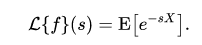
By convention, this is referred to as the Laplace transform of the random variable X itself. Replacing s by −t gives the moment generating function of X. The Laplace transform has applications throughout probability theory, including first passage times of stochastic processes such as Markov chains, and renewal theory.

Of particular use is the ability to recover the cumulative distribution function of a continuous random variable X by means of the Laplace transform as follows

Region of convergence

If f is a locally integrable function (or more generally a Borel measure locally of bounded variation), then the Laplace transform F(s) of f converges provided that the limit

The Laplace transform converges absolutely if the integral

exists (as a proper Lebesgue integral). The Laplace transform is usually understood as conditionally convergent, meaning that it converges in the former instead of the latter sense.

The set of values for which F(s) converges absolutely is either of the form Re(s) > a or else Re(s) ≥ a, where a is an extended real constant, −∞ ≤ a ≤ ∞. (This follows from the dominated convergence theorem.) The constant a is known as the abscissa of absolute convergence, and depends on the growth behavior of f(t). Analogously, the two-sided transform converges absolutely in a strip of the form a < Re(s) < b, and possibly including the lines Re(s) = a or Re(s) = b.The subset of values of s for which the Laplace transform converges absolutely is called the region of absolute convergence or the domain of absolute convergence. In the two-sided case, it is sometimes called the strip of absolute convergence. The Laplace transform is analytic in the region of absolute convergence: this is a consequence of Fubini’s theorem and Morera’s theorem.

Similarly, the set of values for which F(s) converges (conditionally or absolutely) is known as the region of conditional convergence, or simply the region of convergence (ROC). If the Laplace transform converges (conditionally) at s = s0, then it automatically converges for all s with Re(s) > Re(s0). Therefore, the region of convergence is a half-plane of the form Re(s) > a, possibly including some points of the boundary line Re(s) = a.

In the region of convergence Re(s) > Re(s0), the Laplace transform of f can be expressed by integrating by parts as the integral

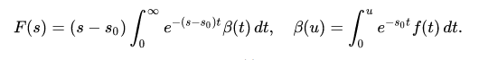
That is, in the region of convergence F(s) can effectively be expressed as the absolutely convergent Laplace transform of some other function. In particular, it is analytic.

There are several Paley–Wiener theorems concerning the relationship between the decay properties of f and the properties of the Laplace transform within the region of convergence.

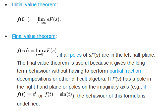
In engineering applications, a function corresponding to a linear time-invariant (LTI) system is stable if every bounded input produces a bounded output. This is equivalent to the absolute convergence of the Laplace transform of the impulse response function in the region Re(s) ≥ 0. As a result, LTI systems are stable provided the poles of the Laplace transform of the impulse response function have negative real part.

This ROC is used in knowing about the causality and stability of a system.

Properties and theorems

The Laplace transform has a number of properties that make it useful for analyzing linear dynamical systems. The most significant advantage is that differentiation and integration become multiplication and division, respectively, by s (similarly to logarithms changing multiplication of numbers to addition of their logarithms).

Because of this property, the Laplace variable s is also known as operator variable in the L domain: either derivative operator or (for s−1) integration operator. The transform turns integral equations and differential equations to polynomial equations, which are much easier to solve. Once solved, use of the inverse Laplace transform reverts to the original domain.

Given the functions f(t) and g(t), and their respective Laplace transforms F(s) and G(s),

Properties of the unilateral Laplace transform

Relation to power series

The Laplace transform can be viewed as a continuous analogue of a power series. If a(n) is a discrete function of a positive integer n, then the power series associated to a(n) is the series

where x is a real variable (see Z transform). Replacing summation over n with integration over t, a continuous version of the power series becomes

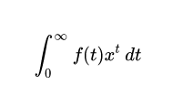
where the discrete function a(n) is replaced by the continuous one f(t).

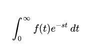
Changing the base of the power from x to e gives

For this to converge for, say, all bounded functions f, it is necessary to require that ln x < 0. Making the substitution −s = ln x gives just the Laplace transform:

In other words, the Laplace transform is a continuous analog of a power series in which the discrete parameter n is replaced by the continuous parameter t, and x is replaced by e−s.

Relation to moments

The quantities

are the moments of the function f. If the first n moments of f converge absolutely, then by repeated differentiation under the integral,

This is of special significance in probability theory, where the moments of a random variable X are given by the expectation values μ n = E ⁡ [ X n ] . Then, the relation holds

Proof of the Laplace transform of a function’s derivative

It is often convenient to use the differentiation property of the Laplace transform to find the transform of a function’s derivative. This can be derived from the basic expression for a Laplace transform as follows:

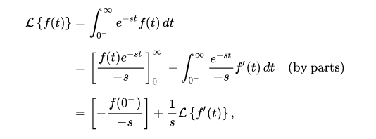
yielding

and in the bilateral case,

The general result

where f ( n )denotes the nth derivative of f, can then be established with an inductive argument.

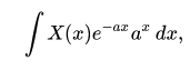
Evaluating integrals over the positive real axis

A useful property of the Laplace transform is the following:

under suitable assumptions on the behaviour of f , g in a right neighbourhood of 0 and on the decay rate of f , g in a left neighbourhood of ∞ . The above formula is a variation of integration by parts, with the operators d d x and ∫ d x being replaced by L and L − 1

. Let us prove the equivalent formulation:

By plugging in

the left-hand side turns into:

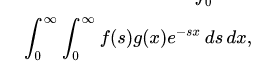
but assuming Fubini’s theorem holds, by reversing the order of integration we get the wanted right-hand side.

Relationship to other transforms

Laplace–Stieltjes transform

The (unilateral) Laplace–Stieltjes transform of a function g : R → R is defined by the Lebesgue–Stieltjes integral

The function g is assumed to be of bounded variation. If g is the antiderivative of f:

then the Laplace–Stieltjes transform of g and the Laplace transform of f coincide. In general, the Laplace–Stieltjes transform is the Laplace transform of the Stieltjes measure associated to g. So in practice, the only distinction between the two transforms is that the Laplace transform is thought of as operating on the density function of the measure, whereas the Laplace–Stieltjes transform is thought of as operating on its cumulative distribution function.

Fourier transform

The continuous Fourier transform is equivalent to evaluating the bilateral Laplace transform with imaginary argument s = iω or s = 2πfi[24] when the condition explained below is fulfilled,

This definition of the Fourier transform requires a prefactor of 1/2 π on the reverse Fourier transform. This relationship between the Laplace and Fourier transforms is often used to determine the frequency spectrum of a signal or dynamical system.

The above relation is valid as stated if and only if the region of convergence (ROC) of F(s) contains the imaginary axis, σ = 0.

For example, the function f(t) = cos(ω0t) has a Laplace transform F(s) = s/(s2 + ω02) whose ROC is Re(s) > 0. As s = iω is a pole of F(s), substituting s = iω in F(s) does not yield the Fourier transform of f(t)u(t), which is proportional to the Dirac delta-function δ(ω − ω0).

However, a relation of the form

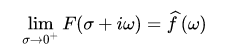
holds under much weaker conditions. For instance, this holds for the above example provided that the limit is understood as a weak limit of measures (see vague topology). General conditions relating the limit of the Laplace transform of a function on the boundary to the Fourier transform take the form of Paley–Wiener theorems.

Mellin transform

The Mellin transform and its inverse are related to the two-sided Laplace transform by a simple change of variables.

If in the Mellin transform

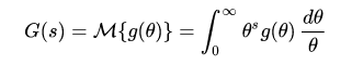
we set θ = e−t we get a two-sided Laplace transform.

Z-transform

The unilateral or one-sided Z-transform is simply the Laplace transform of an ideally sampled signal with the substitution of

where T = 1/fs is the sampling period (in units of time e.g., seconds) and fs is the sampling rate (in samples per second or hertz).

Let

be a sampling impulse train (also called a Dirac comb) and

be the sampled representation of the continuous-time x(t)

The Laplace transform of the sampled signal x_q(t) is

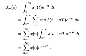
This is the precise definition of the unilateral Z-transform of the discrete function x[n]

with the substitution of z → esT.

Comparing the last two equations, we find the relationship between the unilateral Z-transform and the Laplace transform of the sampled signal,

The similarity between the Z and Laplace transforms is expanded upon in the theory of time scale calculus.

Borel transform

The integral form of the Borel transform

is a special case of the Laplace transform for f an entire function of exponential type, meaning that

for some constants A and B. The generalized Borel transform allows a different weighting function to be used, rather than the exponential function, to transform functions not of exponential type. Nachbin’s theorem gives necessary and sufficient conditions for the Borel transform to be well defined.

Fundamental relationships

Since an ordinary Laplace transform can be written as a special case of a two-sided transform, and since the two-sided transform can be written as the sum of two one-sided transforms, the theory of the Laplace-, Fourier-, Mellin-, and Z-transforms are at bottom the same subject. However, a different point of view and different characteristic problems are associated with each of these four major integral transforms.

Table of selected Laplace transforms

The following table provides Laplace transforms for many common functions of a single variable. For definitions and explanations, see the Explanatory Notes at the end of the table.

Because the Laplace transform is a linear operator,

• The Laplace transform of a sum is the sum of Laplace transforms of each term.

• The Laplace transform of a multiple of a function is that multiple times the Laplace transformation of that function.

Using this linearity, and various trigonometric, hyperbolic, and complex number (etc.) properties and/or identities, some Laplace transforms can be obtained from others more quickly than by using the definition directly.

The unilateral Laplace transform takes as input a function whose time domain is the non-negative reals, which is why all of the time domain functions in the table below are multiples of the Heaviside step function, u(t).

The entries of the table that involve a time delay τ are required to be causal (meaning that τ > 0). A causal system is a system where the impulse response h(t) is zero for all time t prior to t = 0. In general, the region of convergence for causal systems is not the same as that of anticausal systems.

s-domain equivalent circuits and impedances

The Laplace transform is often used in circuit analysis, and simple conversions to the s-domain of circuit elements can be made. Circuit elements can be transformed into impedances, very similar to phasor impedances.

Here is a summary of equivalents:

Note that the resistor is exactly the same in the time domain and the s-domain. The sources are put in if there are initial conditions on the circuit elements. For example, if a capacitor has an initial voltage across it, or if the inductor has an initial current through it, the sources inserted in the s-domain account for that.

The equivalents for current and voltage sources are simply derived from the transformations in the table above.