Z-transform

by Dr. Jaydeep T. Vagh

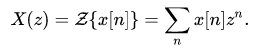
In mathematics and signal processing, the Z-transform converts a discrete-time signal, which is a sequence of real or complex numbers, into a complex frequency-domain representation.

It can be considered as a discrete-time equivalent of the Laplace transform. This similarity is explored in the theory of time-scale calculus.

Definition

The Z-transform can be defined as either a one-sided or two-sided transform.

Bilateral Z-transform

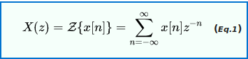
where n is an integer and z is, in general, a complex number:

where A is the magnitude of z j is the imaginary unit, and ϕ is the complex argument (also referred to as angle or phase) in radians.

Unilateral Z-transform

Alternatively, in cases where x [ n ] is defined only for n ≥ 0, the single-sided or unilateral Z-transform is defined as

In signal processing, this definition can be used to evaluate the Z-transform of the unit impulse response of a discrete-time causal system.

An important example of the unilateral Z-transform is the probability-generating function, where the component x [ n ] is the probability that a discrete random variable takes the value n, and the function X ( z ) is usually written as X ( s ) in terms of s = z − 1. The properties of Z-transforms (below) have useful interpretations in the context of probability theory.

Geophysical definition

In geophysics, the usual definition for the Z-transform is a power series in z as opposed to z−1. This convention is used, for example, by Robinson and Treitel and by Kanasewich. The geophysical definition is:

The two definitions are equivalent; however, the difference results in a number of changes. For example, the location of zeros and poles move from inside the unit circle using one definition, to outside the unit circle using the other definition.Thus, care is required to note which definition is being used by a particular author.

Inverse Z-transform

The inverse Z-transform is

where C is a counterclockwise closed path encircling the origin and entirely in the region of convergence (ROC). In the case where the ROC is causal (see Example 2), this means the path C must encircle all of the poles of X ( z ) .

A special case of this contour integral occurs when C is the unit circle. This contour can be used when the ROC includes the unit circle, which is always guaranteed when X ( z ) is stable, that is, when all the poles are inside the unit circle. With this contour, the inverse Z-transform simplifies to the inverse discrete-time Fourier transform, or Fourier series, of the periodic values of the Z-transform around the unit circle:

The Z-transform with a finite range of n and a finite number of uniformly spaced z values can be computed efficiently via Bluestein’s FFT algorithm. The discrete-time Fourier transform (DTFT)—not to be confused with the discrete Fourier transform (DFT)—is a special case of such a Z-transform obtained by restricting z to lie on the unit circle.

Region of convergence

The region of convergence (ROC) is the set of points in the complex plane for which the Z-transform summation converges.

Properties

Parseval’s theorem

Initial value theorem: If x[n] is causal, then

Final value theorem: If the poles of (z−1)X(z) are inside the unit circle, then

Table of common Z-transform pairs

Here

is the unit (or Heaviside) step function and

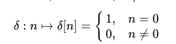
is the discrete-time unit impulse function (cf Dirac delta function which is a continuous-time version). The two functions are chosen together so that the unit step function is the accumulation (running total) of the unit impulse function.

Relationship to Fourier series and Fourier transform

For values of z in the region | z | = 1 , known as the unit circle, we can express the transform as a function of a single, real variable, ω, by defining z = e j ω . And the bi-lateral transform reduces to a Fourier series:

which is also known as the discrete-time Fourier transform (DTFT) of the x [ n ] sequence. This 2π-periodic function is the periodic summation of a Fourier transform, which makes it a widely used analysis tool. To understand this, let X ( f ) be the Fourier transform of any function, x ( t ) , whose samples at some interval, T, equal the x[n] sequence. Then the DTFT of the x[n] sequence can be written as follows.

When T has units of seconds, fhas units of hertz. Comparison of the two series reveals that ω = 2 π f T is a normalized frequency with units of radians per sample. The value ω=2π corresponds to f = 1 T Hz. And now, with the substitution f = ω 2 π T , , Eq.4 can be expressed in terms of the Fourier transform, X(•):

As parameter T changes, the individual terms of Eq.5 move farther apart or closer together along the f-axis. In Eq.6 however, the centers remain 2π apart, while their widths expand or contract. When sequence x(nT) represents the impulse response of an LTI system, these functions are also known as its frequency response. When the x ( n T ) sequence is periodic, its DTFT is divergent at one or more harmonic frequencies, and zero at all other frequencies. This is often represented by the use of amplitude-variant Dirac delta functions at the harmonic frequencies. Due to periodicity, there are only a finite number of unique amplitudes, which are readily computed by the much simpler discrete Fourier transform (DFT). (See DTFT; periodic data.)

Relationship to Laplace transform

Bilinear transform

The bilinear transform can be used to convert continuous-time filters (represented in the Laplace domain) into discrete-time filters (represented in the Z-domain), and vice versa. The following substitution is used:

to convert some function H ( s ) in the Laplace domain to a function H ( z ) H(z) in the Z-domain (Tustin transformation), or

from the Z-domain to the Laplace domain. Through the bilinear transformation, the complex s-plane (of the Laplace transform) is mapped to the complex z-plane (of the z-transform). While this mapping is (necessarily) nonlinear, it is useful in that it maps the entire j ω axis of the s-plane onto the unit circle in the z-plane. As such, the Fourier transform becomes the discrete-time Fourier transform. This assumes that the Fourier transform exists; i.e., that the j ω axis is in the region of convergence of the Laplace transform.

Starred transform

Given a one-sided Z-transform, X(z), of a time-sampled function, the corresponding starred transform produces a Laplace transform and restores the dependence on sampling parameter, T:

The inverse Laplace transform is a mathematical abstraction known as an impulse-sampled function.

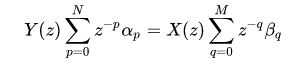
Linear constant-coefficient difference equation

The linear constant-coefficient difference (LCCD) equation is a representation for a linear system based on the autoregressive moving-average equation.

Both sides of the above equation can be divided by α0, if it is not zero, normalizing α0 = 1 and the LCCD equation can be written

This form of the LCCD equation is favorable to make it more explicit that the “current” output y[n] is a function of past outputs y[n−p], current input x[n], and previous inputs x[n−q].

Transfer function

Taking the Z-transform of the above equation (using linearity and time-shifting laws) yields

and rearranging results in

Zeros and poles

From the fundamental theorem of algebra the numerator has M roots (corresponding to zeros of H) and the denominator has N roots (corresponding to poles). Rewriting the transfer function in terms of zeros and poles

where qk is the k-th zero and pk is the k-th pole. The zeros and poles are commonly complex and when plotted on the complex plane (z-plane) it is called the pole–zero plot.

In addition, there may also exist zeros and poles at z = 0 and z = ∞. If we take these poles and zeros as well as multiple-order zeros and poles into consideration, the number of zeros and poles are always equal.

By factoring the denominator, partial fraction decomposition can be used, which can then be transformed back to the time domain. Doing so would result in the impulse response and the linear constant coefficient difference equation of the system.

Output response

If such a system H(z) is driven by a signal X(z) then the output is Y(z) = H(z)X(z). By performing partial fraction decomposition on Y(z) and then taking the inverse Z-transform the output y[n] can be found. In practice, it is often useful to fractionally decompose Y ( z ) before multiplying that quantity by z to generate a form of Y(z) which has terms with easily computable inverse Z-transforms.