Be yourself; Everyone else is already taken.
— Oscar Wilde.
This is the first post on my new blog. I’m just getting this new blog going, so stay tuned for more. Subscribe below to get notified when I post new updates.
Be yourself; Everyone else is already taken.
— Oscar Wilde.
This is the first post on my new blog. I’m just getting this new blog going, so stay tuned for more. Subscribe below to get notified when I post new updates.
By the way, I am going to put blog of quntum computing on this now.
But before that you should know that who were they Hilbert was
Hilber has made a very significant contribution Which shows his talent Quntum computing
Education
At the age of ten, David Hilbert started as a student at the Friedrich Kollegium Gymnasium – a middle school for scholastically accomplished kids, wherever he scanned for a really very long time. In his last middle school year, he was assigned to the additional master math-science Wilhelm Gymnasium.
He graduated at the topmost noteworthy academic level – adequate to scan for a degree at any European school. David Hilbert selected to stay close to home: in 1880, age 18, he enlisted “Albertina” and also looked at mathematics at the University of Konigsberg.
After five years, he had acquired a degree in mathematics and a Ph.D. as well.
| Awards | Lobachevsky Prize (1903) Bolyai Prize (1910) ForMemRS |
|---|
Career
In mid-1882, Hilbert built up a long lasting companionship with the modest, skilled Minkowski.
In 1884, Adolf Hurwitz arrived from Göttingen as an Extraordinarius . An intense and fruitful scientific exchange among the three began, and Minkowski and Hilbert especially would exercise a reciprocal influence over each other at various times in their scientific careers. Hilbert obtained his doctorate in 1885, with a dissertation, written under Ferdinand von Lindemann, titled Über invariante Eigenschaften spezieller binärer Formen, insbesondere der Kugelfunktionen
In 1886 he turned into a mathematics lecturer and then professor at the University of Konigsberg.
Friendly, popularity based and all around adored both as an student and as an instructor, and regularly observed as avoiding the pattern of the formal and elitist arrangement of German science, Hilbert’s numerical virtuoso by the by justified itself with real evidence.
In 1895, as a result of intervention on his behalf by Felix Klein, he obtained the position of Professor of Mathematics at the University of Göttingen. During the Klein and Hilbert years, Göttingen became the preeminent institution in the mathematical world.
At the point when he originally showed up as another teacher at Gottingen he upset the more established educators by heading off to the nearby pool corridor, where he played against his youngsters. He was venerated by his numerous students, whom he tried going on strolls with, so they could discuss mathematical issues casually.
David got the esteemed Bolyai Prize for his eminent work in Mathematics and was accepted as the best mathematician after Poincare.
Work in Mathematics

Contributions
Hilbert built up an expansive scope of crucial thoughts in numerous regions, including invariant hypothesis, the calculus of variations, commutative algebra, arithmetical number hypothesis, the establishments of calculation, and others.
His great works are as follows:-
The Infinite Hotel, a thought experiment created by German mathematician David Hilbert, is a hotel with an infinite number of rooms. Jeff Dekofsky solves these heady lodging issues using Hilbert’s paradox.
Invariant Theory
Hilbert’s first work on invariant capacities drove him to the exhibit in 1888 of his popular limit hypothesis. Twenty years sooner, Paul Gordan had shown the hypothesis of the limit of generators for paired structures utilizing a complex computational methodology.
To tackle what had gotten referred to in certain circles as Gordan’s Problem, Hilbert understood that it was important to take a totally extraordinary way. Therefore, he exhibited Hilbert’s premise hypothesis, demonstrating the presence of a limited arrangement of generators for the invariants of quantics in quite a few factors, however in a theoretical structure.
Hilbert Problems
Hilbert set forth a most compelling rundown of 23 unsolved issues at the International Congress of Mathematicians in Paris in 1900. This is by and large figured as the best and profoundly considered aggregation of open issues actually to be delivered by an individual mathematician.
| Problem | Brief explanation | Status | Year Solved |
|---|---|---|---|
| 1st | The continuum hypothesis (that is, there is no set whose cardinality is strictly between that of the integers and that of the real numbers) | Proven to be impossible to prove or disprove within Zermelo–Fraenkel set theory with or without the Axiom of Choice (provided Zermelo–Fraenkel set theory is consistent, i.e., it does not contain a contradiction). There is no consensus on whether this is a solution to the problem. | 1940, 1963 |
| 2nd | Prove that the axioms of arithmetic are consistent. | There is no consensus on whether results of Gödel and Gentzen give a solution to the problem as stated by Hilbert. Gödel’s second incompleteness theorem, proved in 1931, shows that no proof of its consistency can be carried out within arithmetic itself. Gentzen proved in 1936 that the consistency of arithmetic follows from the well-foundedness of the ordinal ε₀. | 1931, 1936 |
| 3rd | Given any two polyhedra of equal volume, is it always possible to cut the first into finitely many polyhedral pieces that can be reassembled to yield the second? | Resolved. Result: No, proved using Dehn invariants. | 1900 |
| 4th | Construct all metrics where lines are geodesics. | Too vague to be stated resolved or not.[h] | — |
| 5th | Are continuous groups automatically differential groups? | Resolved by Andrew Gleason, assuming one interpretation of the original statement. If, however, it is understood as an equivalent of the Hilbert–Smith conjecture, it is still unsolved. | 1953? |
| 6th | Mathematical treatment of the axioms of physics (a) axiomatic treatment of probability with limit theorems for foundation of statistical physics (b) the rigorous theory of limiting processes “which lead from the atomistic view to the laws of motion of continua” | Partially resolved depending on how the original statement is interpreted.[10] Items (a) and (b) were two specific problems given by Hilbert in a later explanation.[1] Kolmogorov’s axiomatics (1933) is now accepted as standard. There is some success on the way from the “atomistic view to the laws of motion of continua.”[11] | 1933–2002? |
| 7th | Is ab transcendental, for algebraic a ≠ 0,1 and irrational algebraic b ? | Resolved. Result: Yes, illustrated by Gelfond’s theorem or the Gelfond–Schneider theorem. | 1934 |
| 8th | The Riemann hypothesis (“the real part of any non-trivial zero of the Riemann zeta function is ½”) and other prime number problems, among them Goldbach’s conjecture and the twin prime conjecture | Unresolved. | — |
| 9th | Find the most general law of the reciprocity theorem in any algebraic number field. | Partially resolved.[i] | — |
| 10th | Find an algorithm to determine whether a given polynomial Diophantine equation with integer coefficients has an integer solution. | Resolved. Result: Impossible; Matiyasevich’s theorem implies that there is no such algorithm. | 1970 |
| 11th | Solving quadratic forms with algebraic numerical coefficients. | Partially resolved.[12] | — |
| 12th | Extend the Kronecker–Weber theorem on Abelian extensions of the rational numbers to any base number field. | Unresolved. | — |
| 13th | Solve 7th degree equation using algebraic (variant: continuous) functions of two parameters. | Unresolved. The continuous variant of this problem was solved by Vladimir Arnold in 1957 based on work by Andrei Kolmogorov, but the algebraic variant is unresolved.[j] | — |
| 14th | Is the ring of invariants of an algebraic group acting on a polynomial ring always finitely generated? | Resolved. Result: No, a counterexample was constructed by Masayoshi Nagata. | 1959 |
| 15th | Rigorous foundation of Schubert’s enumerative calculus. | Partially resolved.[citation needed] | — |
| 16th | Describe relative positions of ovals originating from a real algebraic curve and as limit cycles of a polynomial vector field on the plane. | Unresolved, even for algebraic curves of degree 8. | — |
| 17th | Express a nonnegative rational function as quotient of sums of squares. | Resolved. Result: Yes, due to Emil Artin. Moreover, an upper limit was established for the number of square terms necessary. | 1927 |
| 18th | (a) Is there a polyhedron that admits only an anisohedral tiling in three dimensions? (b) What is the densest sphere packing? | (a) Resolved. Result: Yes (by Karl Reinhardt). (b) Widely believed to be resolved, by computer-assisted proof (by Thomas Callister Hales). Result: Highest density achieved by close packings, each with density approximately 74%, such as face-centered cubic close packing and hexagonal close packing.[k] | (a) 1928 (b) 1998 |
| 19th | Are the solutions of regular problems in the calculus of variations always necessarily analytic? | Resolved. Result: Yes, proven by Ennio de Giorgi and, independently and using different methods, by John Forbes Nash. | 1957 |
| 20th | Do all variational problems with certain boundary conditions have solutions? | Resolved. A significant topic of research throughout the 20th century, culminating in solutions for the non-linear case. | ? |
| 21st | Proof of the existence of linear differential equations having a prescribed monodromic group | Partially resolved. Result: Yes/No/Open depending on more exact formulations of the problem. | ? |
| 22nd | Uniformization of analytic relations by means of automorphic functions | Partially resolved. Uniformization theorem | ? |
| 23rd | Further development of the calculus of variations | Too vague to be stated resolved or not. | — |
Hilbert began by pulling together all of the many strands of number theory and abstract algebra, before changing the field completely to pursue studies in integral equations, where he revolutionized the then current practices.
In the early 1890s, he developed continuous fractal space-filling curves in multiple dimensions, building on earlier work by Giuseppe Peano. As early as 1899, he proposed a whole new formal set of geometrical axioms, known as Hilbert’s axioms, to substitute the traditional axioms ofEuclid.
But perhaps his greatest legacy is his work on equations, often referred to as his finiteness theorem. He showed that although there were an infinite number of possible equations, it was nevertheless possible to split them up into a finite number of types of equations which could then be used, almost like a set of building blocks, to produce all the other equations.
Hilbert’s Space
Hilbert space is a speculation of the idea of Euclidean space which broadens the techniques for vector variable based math and analytics to spaces with any limited (or even unending) number of measurements.
Hilbert space gave the premise to significant commitments to the arithmetic of material science over the next many years, may in any case offer extraordinary compared to other numerical definitions of quantum mechanics. Hilbert’s space can be used to study the harmonic of vibrating strings.
Further reading
Sometimes I will make up my mood, I will definitely make a blog on all these problems and I will talk about solutions, but that is enough for now.
Many versions of the official Arduino hardware have been commercially produced to date:[1][2]
| Name | Processor | Format | Host interface | I/O | Release date | Notes | ||||||||||
|---|---|---|---|---|---|---|---|---|---|---|---|---|---|---|---|---|
| Processor | Frequency | Dimensions | Voltage | Flash (KB) | EEPROM (KB) | SRAM (KB) | Digital I/O (pins) | Digital I/O with PWM (pins) | Analog input (pins) | Analog output pins | ||||||
| Arduino Uno WiFi rev 2[3] | ATMEGA4809, NINA-W132 Wi-Fi module from u-blox, ECC608 crypto device | 16 MHz | Arduino / Genuino | 68.6 mm x 53.4 mm [ 2.7 in x 2.1 in ] | USB | 32U4 | 5 V | 48 | 0.25 | 6 | 14 | 5 | 6 | 0 | Announced May 17, 2018 | Contains six-axis accelerometer, gyroscope the NINA/esp32 module supports WiFi and support Bluetooth as Beta feature[4] |
| Arduino / Genuino MKR1000 | ATSAMW25 (made of SAMD21 Cortex-M0+ 32 bit ARM MCU, WINC1500 2.4 GHz 802.11 b/g/n Wi-Fi, and ECC508 crypto device ) | 48 MHz | minimal | 61.5 mm × 25 mm [ 2.4 in × 1.0 in ] | USB | 3.3 V | 256 | No | 32 | 8 | 12 | 7 | 1 | Announced: April 2, 2016 | ||
| Arduino MKR Zero | ATSAMD21G18A | 48 MHz | minimal | USB | 3.3 V | 256 | No | 32 | ||||||||
| Arduino 101[5] Genuino 101 | Intel® Curie™ module[6] two tiny cores, an x86 (Quark SE) and an ARC | 32 MHz | Arduino / Genuino | 68.6 mm × 53.4 mm [ 2.7 in × 2.1 in ] | USB | 3.3 V | 196 | 24 | 14 | 4 | 6 | October 16, 2015 | Contains six-axis accelerometer, gyroscope and Bluetooth | |||
| Arduino Zero[7] | ATSAMD21G18A[8] | 48 MHz | Arduino | 68.6 mm × 53.3 mm [ 2.7 in × 2.1 in ] | USB | Native & EDBG Debug | 3.3 V | 256 | 0 to 16 Kb emulation | 32 | 14 | 12 | 6 | 1 | Released June 15, 2015[9] Announced May 15, 2014[10] Listed on some vendors list Mar 2015 | Beta test started in Aug 1, 2014,[11] 32-bit architecture |
| Arduino Due[12][13] | ATSAM3X8E[14] (Cortex-M3) | 84 MHz | Mega | 101.6 mm × 53.3 mm [ 4 in × 2.1 in ] | USB | 16U2[15] + native host[16] | 3.3 V | 512 | 0[17] | 96 | 54 | 12 | 12 | 2 | October 22, 2012[18] | The first Arduino board based on an ARM Processor. Features 2 channel 12-bit DAC, 84 MHz clock frequency, 32-bit architecture, 512 KB Flash and 96 KB SRAM. Unlike most Arduino boards, it operates on 3.3 V and is not 5 V tolerant. |
| Arduino Yún[19] | Atmega32U4,[20] Atheros AR9331 | 16 MHz, 400 MHz | Arduino | 68.6 mm × 53.3 mm [ 2.7 in × 2.1 in ] | USB | 5 V | 32 KB, 16 MB | 1 KB, 0 KB | 2.5 KB, 64 MB | 14 | 6 | 12 | September 10, 2013[21] | Arduino Yún is the combination of a classic Arduino Leonardo (based on the Atmega32U4 processor) with a WiFi system on a chip (SoC) running Linino, a MIPS GNU/Linux based on OpenWrt. | ||
| Arduino Leonardo[22] | Atmega32U4[20] | 16 MHz | Arduino | 68.6 mm × 53.3 mm [ 2.7 in × 2.1 in ] | USB | 32U4[20] | 5 V | 32 | 1 | 2.5 | 20 | 7 | 12 | July 23, 2012[23] | The Leonardo uses the Atmega32U4 processor, which has a USB controller built-in, eliminating one chip as compared to previous Arduinos. | |
| Arduino Uno[24] | ATmega328P[25] | 16 MHz | Arduino | 68.6 mm × 53.3 mm [ 2.7 in × 2.1 in ] | USB | 8U2[26] (Rev1&2)/ 16U2[15] (Rev3) | 5 V | 32 | 1 | 2 | 14 | 6 | 6 | September 24, 2010[27] | This uses the same ATmega328 as late-model Duemilanove, but whereas the Duemilanove used an FTDI chip for USB, the Uno uses an ATmega16U2 (ATmega8U2 before rev3) programmed as a serial converter. | |
| Arduino Mega2560[28] | ATmega2560[29] | 16 MHz | Mega | 101.6 mm × 53.3 mm [ 4 in × 2.1 in ] | USB | 8U2[26] (Rev1&2)/ 16U2[15] (Rev3) | 5 V | 256 | 4 | 8 | 54 | 15 | 16 | September 24, 2010[27] | Total memory of 256 KB. Uses the ATmega16U2 (ATmega8U2 before Rev3) USB chip. Most shields that were designed for the Duemilanove, Diecimila, or Uno will fit, but a few shields will not fit because of interference with the extra pins. | |
| Arduino Ethernet[30] | ATmega328[31] | 16 MHz | Arduino | 68.6 mm × 53.3 mm [ 2.7 in × 2.1 in ] | Ethernet Serial interface | Wiznet Ethernet | 5 V | 32 | 1 | 2 | 14 | 4 | 6 | July 13, 2011[32] | Based on the same WIZnet W5100 chip as the Arduino Ethernet Shield.[33] A serial interface is provided for programming, but no USB interface. Late versions of this board support Power over Ethernet (PoE). | |
| Arduino Fio[34] | ATmega328P[25] | 8 MHz | minimal | 66.0 mm × 27.9 mm [ 2.6 in × 1.1 in ] | XBee Serial | 3.3 V | 32 | 1 | 2 | 14 | 6 | 8 | March 18, 2010[35] | Includes XBee socket on bottom of board.[34] | ||
| Arduino Nano[36] | ATmega328[31] (ATmega168 before v3.0[37]) | 16 MHz | minimal | 43.18 mm × 18.54 mm [ 1.70 in × 0.73 in ] | USB | FTDI FT232R[38] | 5 V | 16/32 | 0.5/1 | 1/2 | 14 | 6 | 8 | May 15, 2008[39] | This small USB-powered version of the Arduino uses a surface-mounted processor. | |
| LilyPad Arduino[40] | ATmega168V or ATmega328V | 8 MHz | wearable | 51 mm ⌀ [ 2 in ⌀ ] | 2.7-5.5 V | 16 | 0.5 | 1 | 14 | 6 | 6 | October 17, 2007[41] | This minimalist design is for wearable applications. | |||
| Arduino Pro[42] | ATmega168 or ATmega328[42] | 16 MHz | Arduino | 52.1 mm × 53.3 mm [ 2.05 in × 2.1 in ] | UART Serial, I2C(TWI), SPI | FTDI | 5 V or 3.3 V | 16/32 | 0.5/1 | 1/2 | 14 | 6 | 6 | Designed and manufactured by SparkFun Electronics for use in semi-permanent installations. | ||
| Arduino Mega ADK[43] | ATmega2560[29] | 16 MHz | Mega | 101.6 mm × 53.3 mm [ 4 in × 2.1 in ] | 8U2[26] MAX3421E USB Host | 5 V | 256 | 4 | 8 | 54 | 14 | 16 | July 13, 2011[32] | |||
| Arduino Esplora[44] | Atmega32U4[20] | 16 MHz | 165.1 mm × 61.0 mm [ 6.5 in × 2.4 in ] | 32U4[20] | 5 V | 32 | 1 | 2.5 | December 10, 2012 | Analog joystick, four buttons, several sensors, 2 TinkerKit inputs and 2 outputs, LCD connector | ||||||
| Arduino Micro[45] | ATmega32U4[20] | 16 MHz | Mini | 17.8 mm × 48.3 mm [ 0.7 in × 1.9 in ] | 5 V | 32 | 1 | 2.5 | 20 | 7 | 12 | November 8, 2012[46] | This Arduino was co-designed by Adafruit. | |||
| Arduino Pro Mini | ATmega328 | 8 (3.3 V)/16 (5 V) MHz | Mini | 17.8 mm × 33.0 mm [ 0.7 in × 1.3 in ] | Six-pin serial header | 3.3 V / 5 V | 32 | 1 | 2 | 14 | 6 | 6 | Designed and manufactured by SparkFun Electronics. |
Arduino is an open-source platform used for building electronics projects. Arduino consists of both a physical programmable circuit board (often referred to as a microcontroller) and a piece of software, or IDE (Integrated Development Environment) that runs on your computer, used to write and upload computer code to the physical board.
The Arduino platform has become quite popular with people just starting out with electronics, and for good reason. Unlike most previous programmable circuit boards, the Arduino does not need a separate piece of hardware (called a programmer) in order to load new code onto the board — you can simply use a USB cable. Additionally, the Arduino IDE uses a simplified version of C++, making it easier to learn to program. Finally, Arduino provides a standard form factor that breaks out the functions of the micro-controller into a more accessible package.
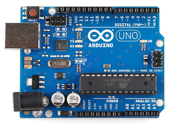
This is an Arduino Uno
The Uno is one of the more popular boards in the Arduino family and a great choice for beginners. We’ll talk about what’s on it and what it can do later in the tutorial.
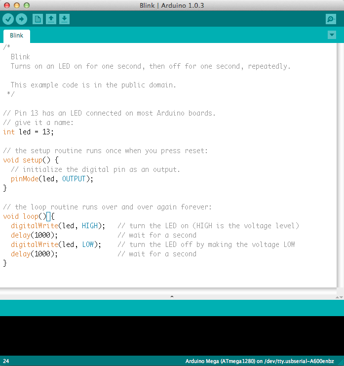
This is a screenshot of the Arduino IDE.
Believe it or not, those 10 lines of code are all you need to blink the on-board LED on your Arduino. The code might not make perfect sense right now, but, after reading this tutorial and the many more Arduino tutorials waiting for you on our site, we’ll get you up to speed in no time!
In this tutorial, we’ll go over the following:
Arduino is a great tool for people of all skill levels. However, you will have a much better time learning along side your Arduino if you understand some basic fundamental electronics beforehand. We recommend that you have at least a decent understanding of these concepts before you dive in to the wonderful world of Arduino.
The Arduino hardware and software was designed for artists, designers, hobbyists, hackers, newbies, and anyone interested in creating interactive objects or environments. Arduino can interact with buttons, LEDs, motors, speakers, GPS units, cameras, the internet, and even your smart-phone or your TV! This flexibility combined with the fact that the Arduino software is free, the hardware boards are pretty cheap, and both the software and hardware are easy to learn has led to a large community of users who have contributed code and released instructions for a huge variety of Arduino-based projects.
For everything from robots and a heating pad hand warming blanket to honest fortune-telling machines, and even a Dungeons and Dragons dice-throwing gauntlet, the Arduino can be used as the brains behind almost any electronics project.

_Wear your nerd cred on your sleev… err, arm. _
And that’s really just the tip of the iceberg — if you’re curious about where to find more examples of Arduino projects in action, here are some good resources for Arduino-based projects to get your creative juices flowing:
There are many varieties of Arduino boards (explained on the next page) that can be used for different purposes. Some boards look a bit different from the one below, but most Arduinos have the majority of these components in common:
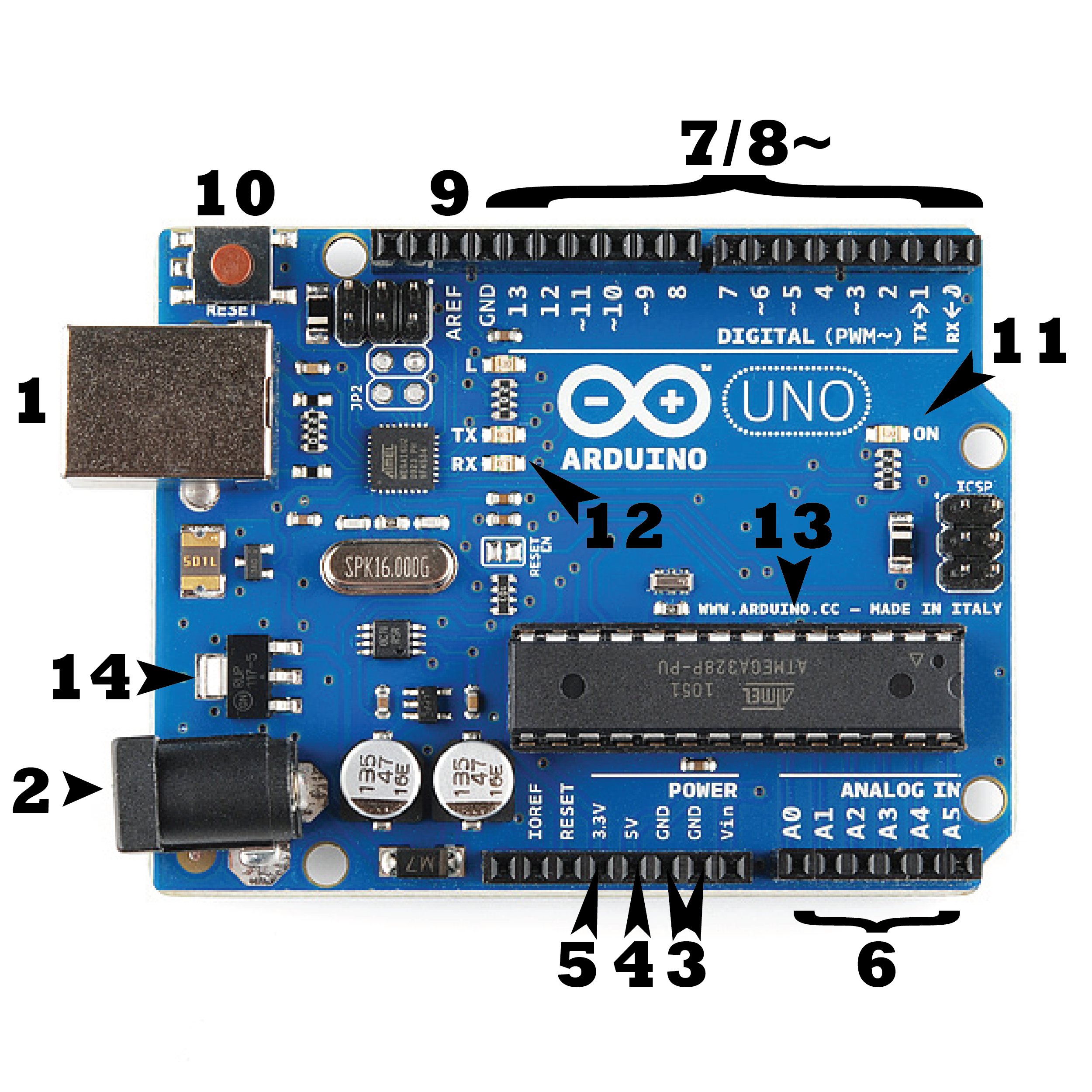
Every Arduino board needs a way to be connected to a power source. The Arduino UNO can be powered from a USB cable coming from your computer or a wall power supply (like this) that is terminated in a barrel jack. In the picture above the USB connection is labeled (1) and the barrel jack is labeled (2).
The USB connection is also how you will load code onto your Arduino board. More on how to program with Arduino can be found in our Installing and Programming Arduino tutorial.
NOTE: Do NOT use a power supply greater than 20 Volts as you will overpower (and thereby destroy) your Arduino. The recommended voltage for most Arduino models is between 6 and 12 Volts.
The pins on your Arduino are the places where you connect wires to construct a circuit (probably in conjuction with a breadboard and some wire. They usually have black plastic ‘headers’ that allow you to just plug a wire right into the board. The Arduino has several different kinds of pins, each of which is labeled on the board and used for different functions.
Just like the original Nintendo, the Arduino has a reset button (10). Pushing it will temporarily connect the reset pin to ground and restart any code that is loaded on the Arduino. This can be very useful if your code doesn’t repeat, but you want to test it multiple times. Unlike the original Nintendo however, blowing on the Arduino doesn’t usually fix any problems.
Just beneath and to the right of the word “UNO” on your circuit board, there’s a tiny LED next to the word ‘ON’ (11). This LED should light up whenever you plug your Arduino into a power source. If this light doesn’t turn on, there’s a good chance something is wrong. Time to re-check your circuit!
TX is short for transmit, RX is short for receive. These markings appear quite a bit in electronics to indicate the pins responsible for serial communication. In our case, there are two places on the Arduino UNO where TX and RX appear — once by digital pins 0 and 1, and a second time next to the TX and RX indicator LEDs (12). These LEDs will give us some nice visual indications whenever our Arduino is receiving or transmitting data (like when we’re loading a new program onto the board).
The black thing with all the metal legs is an IC, or Integrated Circuit (13). Think of it as the brains of our Arduino. The main IC on the Arduino is slightly different from board type to board type, but is usually from the ATmega line of IC’s from the ATMEL company. This can be important, as you may need to know the IC type (along with your board type) before loading up a new program from the Arduino software. This information can usually be found in writing on the top side of the IC. If you want to know more about the difference between various IC’s, reading the datasheets is often a good idea.
The voltage regulator (14) is not actually something you can (or should) interact with on the Arduino. But it is potentially useful to know that it is there and what it’s for. The voltage regulator does exactly what it says — it controls the amount of voltage that is let into the Arduino board. Think of it as a kind of gatekeeper; it will turn away an extra voltage that might harm the circuit. Of course, it has its limits, so don’t hook up your Arduino to anything greater than 20 volts.
With some simple code, the Arduino can control and interact with a wide variety of sensors – things that can measure light, temperature, degree of flex, pressure, proximity, acceleration, carbon monoxide, radioactivity, humidity, barometric pressure, you name it, you can sense it!
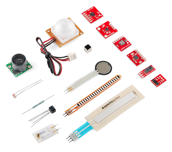
Just a few of the sensors that are easily compatible with Arduino
Additionally, there are these things called shields — basically they are pre-built circuit boards that fit on top of your Arduino and provide additional capabilities — controlling motors, connecting to the internet, providing cellular or other wireless communication, controlling an LCD screen, and much more.
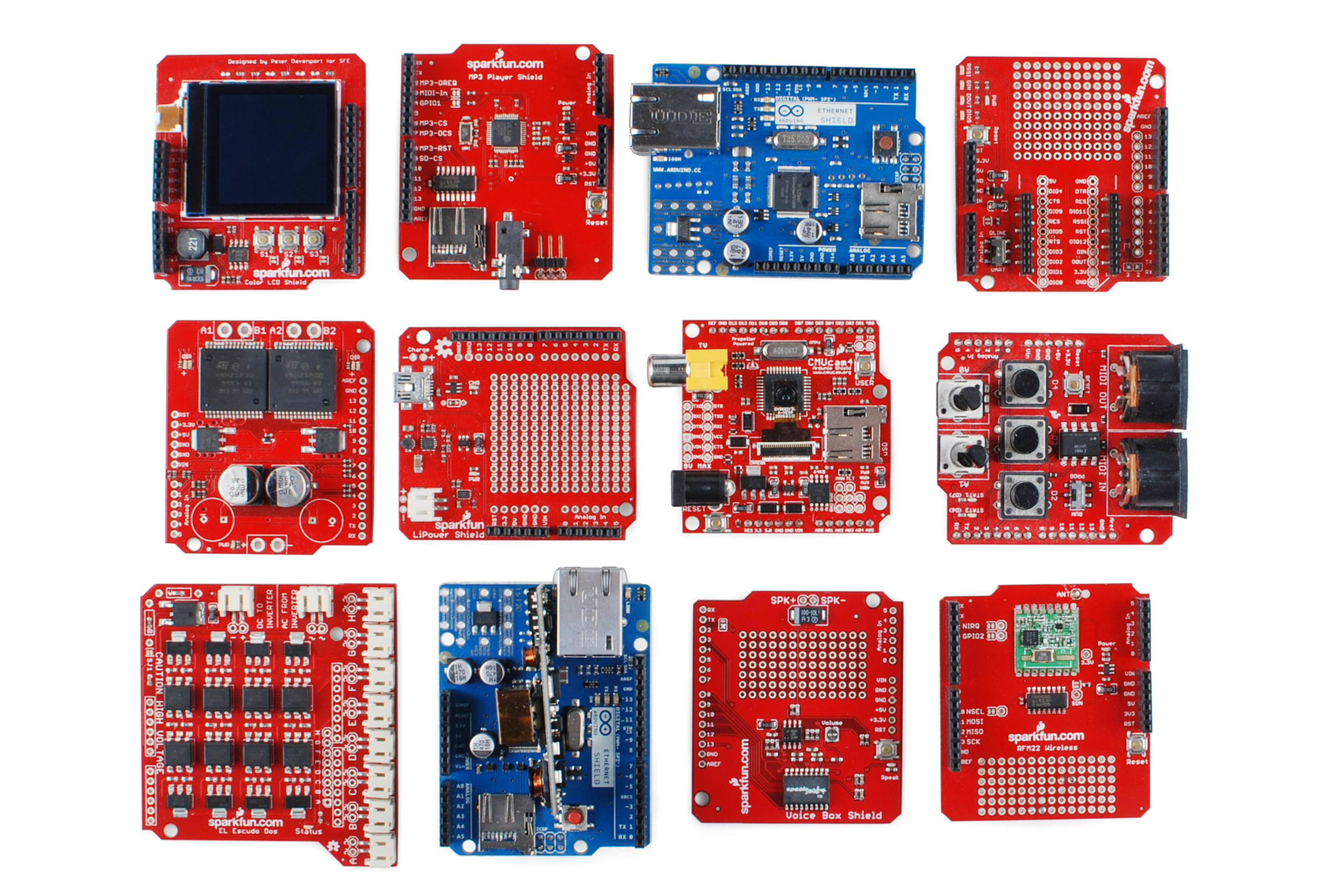
A partial selection of available shields to extend the power of your Arduino
For more on shields, check out:
by Dr. Jaydeep T. Vagh
“AI” redirects here. For other uses, see AI (disambiguation) and Artificial intelligence (disambiguation).
In computer science, artificial intelligence (AI), sometimes called machine intelligence, is intelligence demonstrated by machines, in contrast to the natural intelligence displayed by humans. Colloquially, the term “artificial intelligence” is often used to describe machines (or computers) that mimic “cognitive” functions that humans associate with the human mind, such as “learning” and “problem solving”.
As machines become increasingly capable, tasks considered to require “intelligence” are often removed from the definition of AI, a phenomenon known as the AI effect. A quip in Tesler’s Theorem says “AI is whatever hasn’t been done yet.” For instance, optical character recognition is frequently excluded from things considered to be AI, having become a routine technology.[4] Modern machine capabilities generally classified as AI include successfully understanding human speech, competing at the highest level in strategic game systems (such as chess and Go). autonomously operating cars, intelligent routing in content delivery networks, and military simulations.
Artificial intelligence can be classified into three different types of systems: analytical, human-inspired, and humanized artificial intelligence. Analytical AI has only characteristics consistent with cognitive intelligence; generating a cognitive representation of the world and using learning based on past experience to inform future decisions. Human-inspired AI has elements from cognitive and emotional intelligence; understanding human emotions, in addition to cognitive elements, and considering them in their decision making. Humanized AI shows characteristics of all types of competencies (i.e., cognitive, emotional, and social intelligence), is able to be self-conscious and is self-aware in interactions.
Artificial intelligence was founded as an academic discipline in 1956, and in the years since has experienced several waves of optimism, followed by disappointment and the loss of funding (known as an “AI winter”), followed by new approaches, success and renewed funding. For most of its history, AI research has been divided into subfields that often fail to communicate with each other.[13] These sub-fields are based on technical considerations, such as particular goals (e.g. “robotics” or “machine learning”), the use of particular tools (“logic” or artificial neural networks), or deep philosophical differences. Subfields have also been based on social factors (particular institutions or the work of particular researchers)
The traditional problems (or goals) of AI research include reasoning, knowledge representation, planning, learning, natural language processing, perception and the ability to move and manipulate objects.[14] General intelligence is among the field’s long-term goals. Approaches include statistical methods, computational intelligence, and traditional symbolic AI. Many tools are used in AI, including versions of search and mathematical optimization, artificial neural networks, and methods based on statistics, probability and economics. The AI field draws upon computer science, information engineering, mathematics, psychology, linguistics, philosophy, and many other fields.
The field was founded on the claim that human intelligence “can be so precisely described that a machine can be made to simulate it”.[19] This raises philosophical arguments about the nature of the mind and the ethics of creating artificial beings endowed with human-like intelligence which are issues that have been explored by myth, fiction and philosophy since antiquity.[20] Some people also consider AI to be a danger to humanity if it progresses unabated.[21] Others believe that AI, unlike previous technological revolutions, will create a risk of mass unemployment.[22]
In the twenty-first century, AI techniques have experienced a resurgence following concurrent advances in computer power, large amounts of data, and theoretical understanding; and AI techniques have become an essential part of the technology industry, helping to solve many challenging problems in computer science, software engineering and operations research
Computer science defines AI research as the study of “intelligent agents“: any device that perceives its environment and takes actions that maximize its chance of successfully achieving its goals. A more elaborate definition characterizes AI as “a system’s ability to correctly interpret external data, to learn from such data, and to use those learnings to achieve specific goals and tasks through flexible adaptation.”
A typical AI analyzes its environment and takes actions that maximize its chance of success. An AI’s intended utility function (or goal) can be simple (“1 if the AI wins a game of Go, 0 otherwise”) or complex (“Do mathematically similar actions to the ones succeeded in the past”). Goals can be explicitly defined, or induced. If the AI is programmed for “reinforcement learning”, goals can be implicitly induced by rewarding some types of behavior or punishing others.[a] Alternatively, an evolutionary system can induce goals by using a “fitness function” to mutate and preferentially replicate high-scoring AI systems, similarly to how animals evolved to innately desire certain goals such as finding food. Some AI systems, such as nearest-neighbor, instead of reason by analogy, these systems are not generally given goals, except to the degree that goals are implicit in their training data. Such systems can still be benchmarked if the non-goal system is framed as a system whose “goal” is to successfully accomplish its narrow classification task.
AI often revolves around the use of algorithms. An algorithm is a set of unambiguous instructions that a mechanical computer can execute. A complex algorithm is often built on top of other, simpler, algorithms. A simple example of an algorithm is the following (optimal for first player) recipe for play at tic-tac-toe
Many AI algorithms are capable of learning from data; they can enhance themselves by learning new heuristics (strategies, or “rules of thumb”, that have worked well in the past), or can themselves write other algorithms. Some of the “learners” described below, including Bayesian networks, decision trees, and nearest-neighbor, could theoretically, (given infinite data, time, and memory) learn to approximate any function, including which combination of mathematical functions would best describe the world[citation needed]. These learners could therefore, derive all possible knowledge, by considering every possible hypothesis and matching them against the data. In practice, it is almost never possible to consider every possibility, because of the phenomenon of “combinatorial explosion”, where the amount of time needed to solve a problem grows exponentially. Much of AI research involves figuring out how to identify and avoid considering broad range of possibilities that are unlikely to be beneficial.[63][64] For example, when viewing a map and looking for the shortest driving route from Denver to New York in the East, one can in most cases skip looking at any path through San Francisco or other areas far to the West; thus, an AI wielding a pathfinding algorithm like A* can avoid the combinatorial explosion that would ensue if every possible route had to be ponderously considered in turn.[65]
The earliest (and easiest to understand) approach to AI was symbolism (such as formal logic): “If an otherwise healthy adult has a fever, then they may have influenza”. A second, more general, approach is Bayesian inference: “If the current patient has a fever, adjust the probability they have influenza in such-and-such way”. The third major approach, extremely popular in routine business AI applications, are analogizers such as SVM and nearest-neighbor: “After examining the records of known past patients whose temperature, symptoms, age, and other factors mostly match the current patient, X% of those patients turned out to have influenza”. A fourth approach is harder to intuitively understand, but is inspired by how the brain’s machinery works: the artificial neural network approach uses artificial “neurons” that can learn by comparing itself to the desired output and altering the strengths of the connections between its internal neurons to “reinforce” connections that seemed to be useful. These four main approaches can overlap with each other and with evolutionary systems; for example, neural nets can learn to make inferences, to generalize, and to make analogies. Some systems implicitly or explicitly use multiple of these approaches, alongside many other AI and non-AI algorithms; the best approach is often different depending on the problem.
Learning algorithms work on the basis that strategies, algorithms, and inferences that worked well in the past are likely to continue working well in the future. These inferences can be obvious, such as “since the sun rose every morning for the last 10,000 days, it will probably rise tomorrow morning as well”. They can be nuanced, such as “X% of families have geographically separate species with color variants, so there is an Y% chance that undiscovered black swans exist”. Learners also work on the basis of “Occam’s razor”: The simplest theory that explains the data is the likeliest. Therefore, according to Occam’s razor principle, a learner must be designed such that it prefers simpler theories to complex theories, except in cases where the complex theory is proven substantially better.
Settling on a bad, overly complex theory gerrymandered to fit all the past training data is known as overfitting. Many systems attempt to reduce overfitting by rewarding a theory in accordance with how well it fits the data, but penalizing the theory in accordance with how complex the theory is. Besides classic overfitting, learners can also disappoint by “learning the wrong lesson”. A toy example is that an image classifier trained only on pictures of brown horses and black cats might conclude that all brown patches are likely to be horses. A real-world example is that, unlike humans, current image classifiers don’t determine the spatial relationship between components of the picture; instead, they learn abstract patterns of pixels that humans are oblivious to, but that linearly correlate with images of certain types of real objects. Faintly superimposing such a pattern on a legitimate image results in an “adversarial” image that the system misclassifies.
Compared with humans, existing AI lacks several features of human “commonsense reasoning”; most notably, humans have powerful mechanisms for reasoning about “naïve physics” such as space, time, and physical interactions. This enables even young children to easily make inferences like “If I roll this pen off a table, it will fall on the floor”. Humans also have a powerful mechanism of “folk psychology” that helps them to interpret natural-language sentences such as “The city councilmen refused the demonstrators a permit because they advocated violence”. (A generic AI has difficulty discerning whether the ones alleged to be advocating violence are the councilmen or the demonstrators.) This lack of “common knowledge” means that AI often makes different mistakes than humans make, in ways that can seem incomprehensible. For example, existing self-driving cars cannot reason about the location nor the intentions of pedestrians in the exact way that humans do, and instead must use non-human modes of reasoning to avoid accidents.
The overall research goal of artificial intelligence is to create technology that allows computers and machines to function in an intelligent manner. The general problem of simulating (or creating) intelligence has been broken down into sub-problems. These consist of particular traits or capabilities that researchers expect an intelligent system to display. The traits described below have received the most attention.
Early researchers developed algorithms that imitated step-by-step reasoning that humans use when they solve puzzles or make logical deductions.[82] By the late 1980s and 1990s, AI research had developed methods for dealing with uncertain or incomplete information, employing concepts from probability and economics.
These algorithms proved to be insufficient for solving large reasoning problems, because they experienced a “combinatorial explosion”: they became exponentially slower as the problems grew larger. In fact, even humans rarely use the step-by-step deduction that early AI research was able to model. They solve most of their problems using fast, intuitive judgements.
Knowledge representation and knowledge engineering are central to classical AI research. Some “expert systems” attempt to gather together explicit knowledge possessed by experts in some narrow domain. In addition, some projects attempt to gather the “commonsense knowledge” known to the average person into a database containing extensive knowledge about the world. Among the things a comprehensive commonsense knowledge base would contain are: objects, properties, categories and relations between objects; situations, events, states and time; causes and effects; knowledge about knowledge (what we know about what other people know); and many other, less well researched domains. A representation of “what exists” is an ontology: the set of objects, relations, concepts, and properties formally described so that software agents can interpret them. The semantics of these are captured as description logic concepts, roles, and individuals, and typically implemented as classes, properties, and individuals in the Web Ontology Language. The most general ontologies are called upper ontologies, which attempt to provide a foundation for all other knowledge by acting as mediators between domain ontologies that cover specific knowledge about a particular knowledge domain (field of interest or area of concern). Such formal knowledge representations can be used in content-based indexing and retrieval, scene interpretation, clinical decision support, knowledge discovery (mining “interesting” and actionable inferences from large databases), and other areas.
Among the most difficult problems in knowledge representation are: Default reasoning and the qualification problem Many of the things people know take the form of “working assumptions”. For example, if a bird comes up in conversation, people typically picture an animal that is fist-sized, sings, and flies. None of these things are true about all birds. John McCarthy identified this problem in 1969 as the qualification problem: for any commonsense rule that AI researchers care to represent, there tend to be a huge number of exceptions. Almost nothing is simply true or false in the way that abstract logic requires. AI research has explored a number of solutions to this problem. The breadth of commonsense knowledge The number of atomic facts that the average person knows is very large. Research projects that attempt to build a complete knowledge base of commonsense knowledge (e.g., Cyc) require enormous amounts of laborious ontological engineering—they must be built, by hand, one complicated concept at a time. The subsymbolic form of some commonsense knowledge Much of what people know is not represented as “facts” or “statements” that they could express verbally. For example, a chess master will avoid a particular chess position because it “feels too exposed” or an art critic can take one look at a statue and realize that it is a fake. These are non-conscious and sub-symbolic intuitions or tendencies in the human brain. Knowledge like this informs, supports and provides a context for symbolic, conscious knowledge. As with the related problem of sub-symbolic reasoning, it is hoped that situated AI, computational intelligence, or statistical AI will provide ways to represent this kind of knowledge.
Intelligent agents must be able to set goals and achieve them.[104] They need a way to visualize the future—a representation of the state of the world and be able to make predictions about how their actions will change it—and be able to make choices that maximize the utility (or “value”) of available choices.
In classical planning problems, the agent can assume that it is the only system acting in the world, allowing the agent to be certain of the consequences of its actions.However, if the agent is not the only actor, then it requires that the agent can reason under uncertainty. This calls for an agent that can not only assess its environment and make predictions, but also evaluate its predictions and adapt based on its assessment.
Multi-agent planning uses the cooperation and competition of many agents to achieve a given goal. Emergent behavior such as this is used by evolutionary algorithms and swarm intelligence.
Machine learning (ML), a fundamental concept of AI research since the field’s inception,[109] is the study of computer algorithms that improve automatically through experience.
Unsupervised learning is the ability to find patterns in a stream of input, without requiring a human to label the inputs first. Supervised learning includes both classification and numerical regression, which requires a human to label the input data first. Classification is used to determine what category something belongs in, and occurs after a program sees a number of examples of things from several categories. Regression is the attempt to produce a function that describes the relationship between inputs and outputs and predicts how the outputs should change as the inputs change. Both classifiers and regression learners can be viewed as “function approximators” trying to learn an unknown (possibly implicit) function; for example, a spam classifier can be viewed as learning a function that maps from the text of an email to one of two categories, “spam” or “not spam”. Computational learning theory can assess learners by computational complexity, by sample complexity (how much data is required), or by other notions of optimization.In reinforcement learning[113] the agent is rewarded for good responses and punished for bad ones. The agent uses this sequence of rewards and punishments to form a strategy for operating in its problem space.
Natural language processing gives machines the ability to read and understand human language. A sufficiently powerful natural language processing system would enable natural-language user interfaces and the acquisition of knowledge directly from human-written sources, such as newswire texts. Some straightforward applications of natural language processing include information retrieval, text mining, question answering[115] and machine translation.[116] Many current approaches use word co-occurrence frequencies to construct syntactic representations of text. “Keyword spotting” strategies for search are popular and scalable but dumb; a search query for “dog” might only match documents with the literal word “dog” and miss a document with the word “poodle”. “Lexical affinity” strategies use the occurrence of words such as “accident” to assess the sentiment of a document. Modern statistical NLP approaches can combine all these strategies as well as others, and often achieve acceptable accuracy at the page or paragraph level, but continue to lack the semantic understanding required to classify isolated sentences well. Besides the usual difficulties with encoding semantic commonsense knowledge, existing semantic NLP sometimes scales too poorly to be viable in business applications. Beyond semantic NLP, the ultimate goal of “narrative” NLP is to embody a full understanding of commonsense reasoning
Machine perception is the ability to use input from sensors (such as cameras (visible spectrum or infrared), microphones, wireless signals, and active lidar, sonar, radar, and tactile sensors) to deduce aspects of the world. Applications include speech recognition, facial recognition, and object recognition. Computer vision is the ability to analyze visual input. Such input is usually ambiguous; a giant, fifty-meter-tall pedestrian far away may produce exactly the same pixels as a nearby normal-sized pedestrian, requiring the AI to judge the relative likelihood and reasonableness of different interpretations, for example by using its “object model” to assess that fifty-meter pedestrians do not exist.
AI is heavily used in robotics. Advanced robotic arms and other industrial robots, widely used in modern factories, can learn from experience how to move efficiently despite the presence of friction and gear slippage. A modern mobile robot, when given a small, static, and visible environment, can easily determine its location and map its environment; however, dynamic environments, such as (in endoscopy) the interior of a patient’s breathing body, pose a greater challenge. Motion planning is the process of breaking down a movement task into “primitives” such as individual joint movements. Such movement often involves compliant motion, a process where movement requires maintaining physical contact with an object. Moravec’s paradox generalizes that low-level sensorimotor skills that humans take for granted are, counterintuitively, difficult to program into a robot; the paradox is named after Hans Moravec, who stated in 1988 that “it is comparatively easy to make computers exhibit adult level performance on intelligence tests or playing checkers, and difficult or impossible to give them the skills of a one-year-old when it comes to perception and mobility”. This is attributed to the fact that, unlike checkers, physical dexterity has been a direct target of natural selection for millions of years.
Moravec’s paradox can be extended to many forms of social intelligence.[131][132] Distributed multi-agent coordination of autonomous vehicles remains a difficult problem.[133] Affective computing is an interdisciplinary umbrella that comprises systems which recognize, interpret, process, or simulate human affects. Moderate successes related to affective computing include textual sentiment analysis and, more recently, multimodal affect analysis (see multimodal sentiment analysis), wherein AI classifies the affects displayed by a videotaped subject.
In the long run, social skills and an understanding of human emotion and game theory would be valuable to a social agent. Being able to predict the actions of others by understanding their motives and emotional states would allow an agent to make better decisions. Some computer systems mimic human emotion and expressions to appear more sensitive to the emotional dynamics of human interaction, or to otherwise facilitate human–computer interaction. Similarly, some virtual assistants are programmed to speak conversationally or even to banter humorously; this tends to give naïve users an unrealistic conception of how intelligent existing computer agents actually are.
Historically, projects such as the Cyc knowledge base (1984–) and the massive Japanese Fifth Generation Computer Systems initiative (1982–1992) attempted to cover the breadth of human cognition. These early projects failed to escape the limitations of non-quantitative symbolic logic models and, in retrospect, greatly underestimated the difficulty of cross-domain AI. Nowadays, the vast majority of current AI researchers work instead on tractable “narrow AI” applications (such as medical diagnosis or automobile navigation). Many researchers predict that such “narrow AI” work in different individual domains will eventually be incorporated into a machine with artificial general intelligence (AGI), combining most of the narrow skills mentioned in this article and at some point even exceeding human ability in most or all these areas. Many advances have general, cross-domain significance. One high-profile example is that DeepMind in the 2010s developed a “generalized artificial intelligence” that could learn many diverse Atari games on its own, and later developed a variant of the system which succeeds at sequential learning. Besides transfer learning, hypothetical AGI breakthroughs could include the development of reflective architectures that can engage in decision-theoretic metareasoning, and figuring out how to “slurp up” a comprehensive knowledge base from the entire unstructured Web. Some argue that some kind of (currently-undiscovered) conceptually straightforward, but mathematically difficult, “Master Algorithm” could lead to AGI. Finally, a few “emergent” approaches look to simulating human intelligence extremely closely, and believe that anthropomorphic features like an artificial brain or simulated child development may someday reach a critical point where general intelligence emerges.
Many of the problems in this article may also require general intelligence, if machines are to solve the problems as well as people do. For example, even specific straightforward tasks, like machine translation, require that a machine read and write in both languages (NLP), follow the author’s argument (reason), know what is being talked about (knowledge), and faithfully reproduce the author’s original intent (social intelligence). A problem like machine translation is considered “AI-complete”, because all of these problems need to be solved simultaneously in order to reach human-level machine performance.
There is no established unifying theory or paradigm that guides AI research. Researchers disagree about many issues. A few of the most long standing questions that have remained unanswered are these: should artificial intelligence simulate natural intelligence by studying psychology or neurobiology? Or is human biology as irrelevant to AI research as bird biology is to aeronautical engineering? Can intelligent behavior be described using simple, elegant principles (such as logic or optimization)? Or does it necessarily require solving a large number of completely unrelated problems?
In the 1940s and 1950s, a number of researchers explored the connection between neurobiology, information theory, and cybernetics. Some of them built machines that used electronic networks to exhibit rudimentary intelligence, such as W. Grey Walter’s turtles and the Johns Hopkins Beast. Many of these researchers gathered for meetings of the Teleological Society at Princeton University and the Ratio Club in England. By 1960, this approach was largely abandoned, although elements of it would be revived in the 1980s.
When access to digital computers became possible in the mid 1950s, AI research began to explore the possibility that human intelligence could be reduced to symbol manipulation. The research was centered in three institutions: Carnegie Mellon University, Stanford and MIT, and as described below, each one developed its own style of research. John Haugeland named these symbolic approaches to AI “good old fashioned AI” or “GOFAI“. During the 1960s, symbolic approaches had achieved great success at simulating high-level thinking in small demonstration programs. Approaches based on cybernetics or artificial neural networks were abandoned or pushed into the background. Researchers in the 1960s and the 1970s were convinced that symbolic approaches would eventually succeed in creating a machine with artificial general intelligence and considered this the goal of their field.
Economist Herbert Simon and Allen Newell studied human problem-solving skills and attempted to formalize them, and their work laid the foundations of the field of artificial intelligence, as well as cognitive science, operations research and management science. Their research team used the results of psychological experiments to develop programs that simulated the techniques that people used to solve problems. This tradition, centered at Carnegie Mellon University would eventually culminate in the development of the Soar architecture in the middle 1980s.
Unlike Simon and Newell, John McCarthy felt that machines did not need to simulate human thought, but should instead try to find the essence of abstract reasoning and problem-solving, regardless whether people used the same algorithms. His laboratory at Stanford (SAIL) focused on using formal logic to solve a wide variety of problems, including knowledge representation, planning and learning. Logic was also the focus of the work at the University of Edinburgh and elsewhere in Europe which led to the development of the programming language Prolog and the science of logic programming.
Researchers at MIT (such as Marvin Minsky and Seymour Papert) found that solving difficult problems in vision and natural language processing required ad-hoc solutions—they argued that there was no simple and general principle (like logic) that would capture all the aspects of intelligent behavior. Roger Schank described their “anti-logic” approaches as “scruffy” (as opposed to the “neat” paradigms at CMU and Stanford). Commonsense knowledge bases (such as Doug Lenat‘s Cyc) are an example of “scruffy” AI, since they must be built by hand, one complicated concept at a time.
When computers with large memories became available around 1970, researchers from all three traditions began to build knowledge into AI applications. This “knowledge revolution” led to the development and deployment of expert systems (introduced by Edward Feigenbaum), the first truly successful form of AI software. A key component of the system architecture for all expert systems is the knowledge base, which stores facts and rules that illustrate AI. The knowledge revolution was also driven by the realization that enormous amounts of knowledge would be required by many simple AI applications.
By the 1980s, progress in symbolic AI seemed to stall and many believed that symbolic systems would never be able to imitate all the processes of human cognition, especially perception, robotics, learning and pattern recognition. A number of researchers began to look into “sub-symbolic” approaches to specific AI problems. Sub-symbolic methods manage to approach intelligence without specific representations of knowledge.
This includes embodied, situated, behavior-based, and nouvelle AI. Researchers from the related field of robotics, such as Rodney Brooks, rejected symbolic AI and focused on the basic engineering problems that would allow robots to move and survive. Their work revived the non-symbolic point of view of the early cybernetics researchers of the 1950s and reintroduced the use of control theory in AI. This coincided with the development of the embodied mind thesis in the related field of cognitive science: the idea that aspects of the body (such as movement, perception and visualization) are required for higher intelligence.
Within developmental robotics, developmental learning approaches are elaborated upon to allow robots to accumulate repertoires of novel skills through autonomous self-exploration, social interaction with human teachers, and the use of guidance mechanisms (active learning, maturation, motor synergies, etc.).
Interest in neural networks and “connectionism” was revived by David Rumelhart and others in the middle of the 1980s. Artificial neural networks are an example of soft computing—they are solutions to problems which cannot be solved with complete logical certainty, and where an approximate solution is often sufficient. Other soft computing approaches to AI include fuzzy systems, Grey system theory, evolutionary computation and many statistical tools. The application of soft computing to AI is studied collectively by the emerging discipline of computational intelligence.
Much of traditional GOFAI got bogged down on ad hoc patches to symbolic computation that worked on their own toy models but failed to generalize to real-world results. However, around the 1990s, AI researchers adopted sophisticated mathematical tools, such as hidden Markov models (HMM), information theory, and normative Bayesian decision theory to compare or to unify competing architectures. The shared mathematical language permitted a high level of collaboration with more established fields (like mathematics, economics or operations research). Compared with GOFAI, new “statistical learning” techniques such as HMM and neural networks were gaining higher levels of accuracy in many practical domains such as data mining, without necessarily acquiring a semantic understanding of the datasets. The increased successes with real-world data led to increasing emphasis on comparing different approaches against shared test data to see which approach performed best in a broader context than that provided by idiosyncratic toy models; AI research was becoming more scientific. Nowadays results of experiments are often rigorously measurable, and are sometimes (with difficulty) reproducible.Different statistical learning techniques have different limitations; for example, basic HMM cannot model the infinite possible combinations of natural language. Critics note that the shift from GOFAI to statistical learning is often also a shift away from explainable AI. In AGI research, some scholars caution against over-reliance on statistical learning, and argue that continuing research into GOFAI will still be necessary to attain general intelligence.
Intelligent agent paradigm An intelligent agent is a system that perceives its environment and takes actions which maximize its chances of success. The simplest intelligent agents are programs that solve specific problems. More complicated agents include human beings and organizations of human beings (such as firms). The paradigm allows researchers to directly compare or even combine different approaches to isolated problems, by asking which agent is best at maximizing a given “goal function”. An agent that solves a specific problem can use any approach that works—some agents are symbolic and logical, some are sub-symbolic artificial neural networks and others may use new approaches. The paradigm also gives researchers a common language to communicate with other fields—such as decision theory and economics—that also use concepts of abstract agents. Building a complete agent requires researchers to address realistic problems of integration; for example, because sensory systems give uncertain information about the environment, planning systems must be able to function in the presence of uncertainty. The intelligent agent paradigm became widely accepted during the 1990s.Agent architectures and cognitive architectures Researchers have designed systems to build intelligent systems out of interacting intelligent agents in a multi-agent system. A hierarchical control system provides a bridge between sub-symbolic AI at its lowest, reactive levels and traditional symbolic AI at its highest levels, where relaxed time constraints permit planning and world modelling. Some cognitive architectures are custom-built to solve a narrow problem; others, such as Soar, are designed to mimic human cognition and to provide insight into general intelligence. Modern extensions of Soar are hybrid intelligent systems that include both symbolic and sub-symbolic components.
AI has developed a large number of tools to solve the most difficult problems in computer science. A few of the most general of these methods are discussed below.
Many problems in AI can be solved in theory by intelligently searching through many possible solutions: Reasoning can be reduced to performing a search. For example, logical proof can be viewed as searching for a path that leads from premises to conclusions, where each step is the application of an inference rule. Planning algorithms search through trees of goals and subgoals, attempting to find a path to a target goal, a process called means-ends analysis.Robotics algorithms for moving limbs and grasping objects use local searches in configuration space. Many learning algorithms use search algorithms based on optimization.
Simple exhaustive searches are rarely sufficient for most real-world problems: the search space (the number of places to search) quickly grows to astronomical numbers. The result is a search that is too slow or never completes. The solution, for many problems, is to use “heuristics” or “rules of thumb” that prioritize choices in favor of those that are more likely to reach a goal and to do so in a shorter number of steps. In some search methodologies heuristics can also serve to entirely eliminate some choices that are unlikely to lead to a goal (called “pruning the search tree“). Heuristics supply the program with a “best guess” for the path on which the solution lies. Heuristics limit the search for solutions into a smaller sample size.
A very different kind of search came to prominence in the 1990s, based on the mathematical theory of optimization. For many problems, it is possible to begin the search with some form of a guess and then refine the guess incrementally until no more refinements can be made. These algorithms can be visualized as blind hill climbing: we begin the search at a random point on the landscape, and then, by jumps or steps, we keep moving our guess uphill, until we reach the top. Other optimization algorithms are simulated annealing, beam search and random optimization.

A particle swarm seeking the global minimum
Evolutionary computation uses a form of optimization search. For example, they may begin with a population of organisms (the guesses) and then allow them to mutate and recombine, selecting only the fittest to survive each generation (refining the guesses). Classic evolutionary algorithms include genetic algorithms, gene expression programming, and genetic programming. Alternatively, distributed search processes can coordinate via swarm intelligence algorithms. Two popular swarm algorithms used in search are particle swarm optimization (inspired by bird flocking) and ant colony optimization (inspired by ant trails).
Logic is used for knowledge representation and problem solving, but it can be applied to other problems as well. For example, the satplan algorithm uses logic for planning and inductive logic programming is a method for learning.
Several different forms of logic are used in AI research. Propositional logic involves truth functions such as “or” and “not”. First-order logic adds quantifiers and predicates, and can express facts about objects, their properties, and their relations with each other. Fuzzy set theory assigns a “degree of truth” (between 0 and 1) to vague statements such as “Alice is old” (or rich, or tall, or hungry) that are too linguistically imprecise to be completely true or false. Fuzzy logic is successfully used in control systems to allow experts to contribute vague rules such as “if you are close to the destination station and moving fast, increase the train’s brake pressure”; these vague rules can then be numerically refined within the system. Fuzzy logic fails to scale well in knowledge bases; many AI researchers question the validity of chaining fuzzy-logic inferences.
Default logics, non-monotonic logics and circumscription are forms of logic designed to help with default reasoning and the qualification problem. Several extensions of logic have been designed to handle specific domains of knowledge, such as: description logics; situation calculus, event calculus and fluent calculus (for representing events and time); causal calculus; belief calculus; and modal logics.
Overall, qualitative symbolic logic is brittle and scales poorly in the presence of noise or other uncertainty. Exceptions to rules are numerous, and it is difficult for logical systems to function in the presence of contradictory rules.
Many problems in AI (in reasoning, planning, learning, perception, and robotics) require the agent to operate with incomplete or uncertain information. AI researchers have devised a number of powerful tools to solve these problems using methods from probability theory and economics.
Bayesian networks are a very general tool that can be used for a large number of problems: reasoning (using the Bayesian inference algorithm), learning (using the expectation-maximization algorithm), planning (using decision networks)[203] and perception (using dynamic Bayesian networks). Probabilistic algorithms can also be used for filtering, prediction, smoothing and finding explanations for streams of data, helping perception systems to analyze processes that occur over time (e.g., hidden Markov models or Kalman filters). Compared with symbolic logic, formal Bayesian inference is computationally expensive. For inference to be tractable, most observations must be conditionally independent of one another. Complicated graphs with diamonds or other “loops” (undirected cycles) can require a sophisticated method such as Markov chain Monte Carlo, which spreads an ensemble of random walkers throughout the Bayesian network and attempts to converge to an assessment of the conditional probabilities. Bayesian networks are used on Xbox Live to rate and match players; wins and losses are “evidence” of how good a player is. AdSense uses a Bayesian network with over 300 million edges to learn which ads to serve.
A key concept from the science of economics is “utility“: a measure of how valuable something is to an intelligent agent. Precise mathematical tools have been developed that analyze how an agent can make choices and plan, using decision theory, decision analysis, and information value theory. These tools include models such as Markov decision processes, dynamic decision networks, game theory and mechanism design.
Main articles: Classifier (mathematics), Statistical classification, and Machine learning
The simplest AI applications can be divided into two types: classifiers (“if shiny then diamond”) and controllers (“if shiny then pick up”). Controllers do, however, also classify conditions before inferring actions, and therefore classification forms a central part of many AI systems. Classifiers are functions that use pattern matching to determine a closest match. They can be tuned according to examples, making them very attractive for use in AI. These examples are known as observations or patterns. In supervised learning, each pattern belongs to a certain predefined class. A class can be seen as a decision that has to be made. All the observations combined with their class labels are known as a data set. When a new observation is received, that observation is classified based on previous experience.
A classifier can be trained in various ways; there are many statistical and machine learning approaches. The decision tree is perhaps the most widely used machine learning algorithm. Other widely used classifiers are the neural network, k-nearest neighbor algorithm, kernel methods such as the support vector machine (SVM), Gaussian mixture model, and the extremely popular naive Bayes classifier. Classifier performance depends greatly on the characteristics of the data to be classified, such as the dataset size, distribution of samples across classes, the dimensionality, and the level of noise. Model-based classifiers perform well if the assumed model is an extremely good fit for the actual data. Otherwise, if no matching model is available, and if accuracy (rather than speed or scalability) is the sole concern, conventional wisdom is that discriminative classifiers (especially SVM) tend to be more accurate than model-based classifiers such as “naive Bayes” on most practical data sets.
Neural networks were inspired by the architecture of neurons in the human brain. A simple “neuron” N accepts input from multiple other neurons, each of which, when activated (or “fired”), cast a weighted “vote” for or against whether neuron N should itself activate. Learning requires an algorithm to adjust these weights based on the training data; one simple algorithm (dubbed “fire together, wire together“) is to increase the weight between two connected neurons when the activation of one triggers the successful activation of another. The neural network forms “concepts” that are distributed among a subnetwork of shared neurons that tend to fire together; a concept meaning “leg” might be coupled with a subnetwork meaning “foot” that includes the sound for “foot”. Neurons have a continuous spectrum of activation; in addition, neurons can process inputs in a nonlinear way rather than weighing straightforward votes. Modern neural networks can learn both continuous functions and, surprisingly, digital logical operations. Neural networks’ early successes included predicting the stock market and (in 1995) a mostly self-driving car. In the 2010s, advances in neural networks using deep learning thrust AI into widespread public consciousness and contributed to an enormous upshift in corporate AI spending; for example, AI-related M&A in 2017 was over 25 times as large as in 2015.
The study of non-learning artificial neural networks began in the decade before the field of AI research was founded, in the work of Walter Pitts and Warren McCullouch. Frank Rosenblatt invented the perceptron, a learning network with a single layer, similar to the old concept of linear regression. Early pioneers also include Alexey Grigorevich Ivakhnenko, Teuvo Kohonen, Stephen Grossberg, Kunihiko Fukushima, Christoph von der Malsburg, David Willshaw, Shun-Ichi Amari, Bernard Widrow, John Hopfield, Eduardo R. Caianiello, and others[citation needed].
The main categories of networks are acyclic or feedforward neural networks (where the signal passes in only one direction) and recurrent neural networks (which allow feedback and short-term memories of previous input events). Among the most popular feedforward networks are perceptrons, multi-layer perceptrons and radial basis networks. Neural networks can be applied to the problem of intelligent control (for robotics) or learning, using such techniques as Hebbian learning (“fire together, wire together”), GMDH or competitive learning.
Today, neural networks are often trained by the backpropagation algorithm, which had been around since 1970 as the reverse mode of automatic differentiation published by Seppo Linnainmaa, and was introduced to neural networks by Paul Werbos.
Hierarchical temporal memory is an approach that models some of the structural and algorithmic properties of the neocortex.
To summarize, most neural networks use some form of gradient descent on a hand-created neural topology. However, some research groups, such as Uber, argue that simple neuroevolution to mutate new neural network topologies and weights may be competitive with sophisticated gradient descent approaches. One advantage of neuroevolution is that it may be less prone to get caught in “dead ends”.
AI, like electricity or the steam engine, is a general purpose technology. There is no consensus on how to characterize which tasks AI tends to excel at.[263] While projects such as AlphaZero have succeeded in generating their own knowledge from scratch, many other machine learning projects require large training datasets. Researcher Andrew Ng has suggested, as a “highly imperfect rule of thumb”, that “almost anything a typical human can do with less than one second of mental thought, we can probably now or in the near future automate using AI.” Moravec’s paradox suggests that AI lags humans at many tasks that the human brain has specifically evolved to perform well.
Games provide a well-publicized benchmark for assessing rates of progress. AlphaGo around 2016 brought the era of classical board-game benchmarks to a close. Games of imperfect knowledge provide new challenges to AI in the area of game theory. E-sports such as StarCraft continue to provide additional public benchmarks. There are many competitions and prizes, such as the Imagenet Challenge, to promote research in artificial intelligence. The most common areas of competition include general machine intelligence, conversational behavior, data-mining, robotic cars, and robot soccer as well as conventional games.
The “imitation game” (an interpretation of the 1950 Turing test that assesses whether a computer can imitate a human) is nowadays considered too exploitable to be a meaningful benchmark. A derivative of the Turing test is the Completely Automated Public Turing test to tell Computers and Humans Apart (CAPTCHA). As the name implies, this helps to determine that a user is an actual person and not a computer posing as a human. In contrast to the standard Turing test, CAPTCHA is administered by a machine and targeted to a human as opposed to being administered by a human and targeted to a machine. A computer asks a user to complete a simple test then generates a grade for that test. Computers are unable to solve the problem, so correct solutions are deemed to be the result of a person taking the test. A common type of CAPTCHA is the test that requires the typing of distorted letters, numbers or symbols that appear in an image undecipherable by a computer.
Proposed “universal intelligence” tests aim to compare how well machines, humans, and even non-human animals perform on problem sets that are generic as possible. At an extreme, the test suite can contain every possible problem, weighted by Kolmogorov complexity; unfortunately, these problem sets tend to be dominated by impoverished pattern-matching exercises where a tuned AI can easily exceed human performance levels.
AI is relevant to any intellectual task. Modern artificial intelligence techniques are pervasive and are too numerous to list here. Frequently, when a technique reaches mainstream use, it is no longer considered artificial intelligence; this phenomenon is described as the AI effect.
High-profile examples of AI include autonomous vehicles (such as drones and self-driving cars), medical diagnosis, creating art (such as poetry), proving mathematical theorems, playing games (such as Chess or Go), search engines (such as Google search), online assistants (such as Siri), image recognition in photographs, spam filtering, predicting flight delays, prediction of judicial decisions and targeting online advertisements.
With social media sites overtaking TV as a source for news for young people and news organizations increasingly reliant on social media platforms for generating distribution, major publishers now use artificial intelligence (AI) technology to post stories more effectively and generate higher volumes of traffic.
AI is being applied to the high cost problem of dosage issues—where findings suggested that AI could save $16 billion. In 2016, a ground breaking study in California found that a mathematical formula developed with the help of AI correctly determined the accurate dose of immunosuppressant drugs to give to organ patients.

X-ray of a hand, with automatic calculation of bone age by computer software
Artificial intelligence is breaking into the healthcare industry by assisting doctors. According to Bloomberg Technology, Microsoft has developed AI to help doctors find the right treatments for cancer. There is a great amount of research and drugs developed relating to cancer. In detail, there are more than 800 medicines and vaccines to treat cancer. This negatively affects the doctors, because there are too many options to choose from, making it more difficult to choose the right drugs for the patients. Microsoft is working on a project to develop a machine called “Hanover”. Its goal is to memorize all the papers necessary to cancer and help predict which combinations of drugs will be most effective for each patient. One project that is being worked on at the moment is fighting myeloid leukemia, a fatal cancer where the treatment has not improved in decades. Another study was reported to have found that artificial intelligence was as good as trained doctors in identifying skin cancers. Another study is using artificial intelligence to try and monitor multiple high-risk patients, and this is done by asking each patient numerous questions based on data acquired from live doctor to patient interactions. One study was done with transfer learning, the machine performed a diagnosis similarly to a well-trained ophthalmologist, and could generate a decision within 30 seconds on whether or not the patient should be referred for treatment, with more than 95% accuracy.
According to CNN, a recent study by surgeons at the Children’s National Medical Center in Washington successfully demonstrated surgery with an autonomous robot. The team supervised the robot while it performed soft-tissue surgery, stitching together a pig’s bowel during open surgery, and doing so better than a human surgeon, the team claimed. IBM has created its own artificial intelligence computer, the IBM Watson, which has beaten human intelligence (at some levels). Watson not only won at the game show Jeopardy! against former champions, but was declared a hero after successfully diagnosing a woman who was suffering from leukemia.

Advancements in AI have contributed to the growth of the automotive industry through the creation and evolution of self-driving vehicles. As of 2016, there are over 30 companies utilizing AI into the creation of driverless cars. A few companies involved with AI include Tesla, Google, and Apple.
Many components contribute to the functioning of self-driving cars. These vehicles incorporate systems such as braking, lane changing, collision prevention, navigation and mapping. Together, these systems, as well as high performance computers, are integrated into one complex vehicle.
Recent developments in autonomous automobiles have made the innovation of self-driving trucks possible, though they are still in the testing phase. The UK government has passed legislation to begin testing of self-driving truck platoons in 2018. Self-driving truck platoons are a fleet of self-driving trucks following the lead of one non-self-driving truck, so the truck platoons aren’t entirely autonomous yet. Meanwhile, the Daimler, a German automobile corporation, is testing the Freightliner Inspiration which is a semi-autonomous truck that will only be used on the highway.
One main factor that influences the ability for a driver-less automobile to function is mapping. In general, the vehicle would be pre-programmed with a map of the area being driven. This map would include data on the approximations of street light and curb heights in order for the vehicle to be aware of its surroundings. However, Google has been working on an algorithm with the purpose of eliminating the need for pre-programmed maps and instead, creating a device that would be able to adjust to a variety of new surroundings.Some self-driving cars are not equipped with steering wheels or brake pedals, so there has also been research focused on creating an algorithm that is capable of maintaining a safe environment for the passengers in the vehicle through awareness of speed and driving conditions.
Another factor that is influencing the ability for a driver-less automobile is the safety of the passenger. To make a driver-less automobile, engineers must program it to handle high-risk situations. These situations could include a head-on collision with pedestrians. The car’s main goal should be to make a decision that would avoid hitting the pedestrians and saving the passengers in the car. But there is a possibility the car would need to make a decision that would put someone in danger. In other words, the car would need to decide to save the pedestrians or the passengers. The programming of the car in these situations is crucial to a successful driver-less automobile.
by Dr. Jaydeep T. Vagh
In mathematics and signal processing, the Z-transform converts a discrete-time signal, which is a sequence of real or complex numbers, into a complex frequency-domain representation.
It can be considered as a discrete-time equivalent of the Laplace transform. This similarity is explored in the theory of time-scale calculus.
The Z-transform can be defined as either a one-sided or two-sided transform.
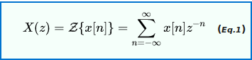
where n is an integer and z is, in general, a complex number:

where A is the magnitude of z j is the imaginary unit, and ϕ is the complex argument (also referred to as angle or phase) in radians.
Alternatively, in cases where x [ n ] is defined only for n ≥ 0, the single-sided or unilateral Z-transform is defined as

In signal processing, this definition can be used to evaluate the Z-transform of the unit impulse response of a discrete-time causal system.
An important example of the unilateral Z-transform is the probability-generating function, where the component x [ n ] is the probability that a discrete random variable takes the value n, and the function X ( z ) is usually written as X ( s ) in terms of s = z − 1. The properties of Z-transforms (below) have useful interpretations in the context of probability theory.
In geophysics, the usual definition for the Z-transform is a power series in z as opposed to z−1. This convention is used, for example, by Robinson and Treitel and by Kanasewich. The geophysical definition is:
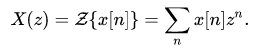
The two definitions are equivalent; however, the difference results in a number of changes. For example, the location of zeros and poles move from inside the unit circle using one definition, to outside the unit circle using the other definition.Thus, care is required to note which definition is being used by a particular author.
The inverse Z-transform is

where C is a counterclockwise closed path encircling the origin and entirely in the region of convergence (ROC). In the case where the ROC is causal (see Example 2), this means the path C must encircle all of the poles of X ( z ) .
A special case of this contour integral occurs when C is the unit circle. This contour can be used when the ROC includes the unit circle, which is always guaranteed when X ( z ) is stable, that is, when all the poles are inside the unit circle. With this contour, the inverse Z-transform simplifies to the inverse discrete-time Fourier transform, or Fourier series, of the periodic values of the Z-transform around the unit circle:

The Z-transform with a finite range of n and a finite number of uniformly spaced z values can be computed efficiently via Bluestein’s FFT algorithm. The discrete-time Fourier transform (DTFT)—not to be confused with the discrete Fourier transform (DFT)—is a special case of such a Z-transform obtained by restricting z to lie on the unit circle.
The region of convergence (ROC) is the set of points in the complex plane for which the Z-transform summation converges.


Parseval’s theorem

Initial value theorem: If x[n] is causal, then

Final value theorem: If the poles of (z−1)X(z) are inside the unit circle, then

Here

is the unit (or Heaviside) step function and
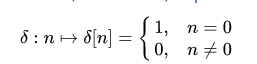
is the discrete-time unit impulse function (cf Dirac delta function which is a continuous-time version). The two functions are chosen together so that the unit step function is the accumulation (running total) of the unit impulse function.


For values of z in the region | z | = 1 , known as the unit circle, we can express the transform as a function of a single, real variable, ω, by defining z = e j ω . And the bi-lateral transform reduces to a Fourier series:

which is also known as the discrete-time Fourier transform (DTFT) of the x [ n ] sequence. This 2π-periodic function is the periodic summation of a Fourier transform, which makes it a widely used analysis tool. To understand this, let X ( f ) be the Fourier transform of any function, x ( t ) , whose samples at some interval, T, equal the x[n] sequence. Then the DTFT of the x[n] sequence can be written as follows.

When T has units of seconds, fhas units of hertz. Comparison of the two series reveals that ω = 2 π f T is a normalized frequency with units of radians per sample. The value ω=2π corresponds to f = 1 T Hz. And now, with the substitution f = ω 2 π T , , Eq.4 can be expressed in terms of the Fourier transform, X(•):

As parameter T changes, the individual terms of Eq.5 move farther apart or closer together along the f-axis. In Eq.6 however, the centers remain 2π apart, while their widths expand or contract. When sequence x(nT) represents the impulse response of an LTI system, these functions are also known as its frequency response. When the x ( n T ) sequence is periodic, its DTFT is divergent at one or more harmonic frequencies, and zero at all other frequencies. This is often represented by the use of amplitude-variant Dirac delta functions at the harmonic frequencies. Due to periodicity, there are only a finite number of unique amplitudes, which are readily computed by the much simpler discrete Fourier transform (DFT). (See DTFT; periodic data.)
The bilinear transform can be used to convert continuous-time filters (represented in the Laplace domain) into discrete-time filters (represented in the Z-domain), and vice versa. The following substitution is used:

to convert some function H ( s ) in the Laplace domain to a function H ( z ) H(z) in the Z-domain (Tustin transformation), or

from the Z-domain to the Laplace domain. Through the bilinear transformation, the complex s-plane (of the Laplace transform) is mapped to the complex z-plane (of the z-transform). While this mapping is (necessarily) nonlinear, it is useful in that it maps the entire j ω axis of the s-plane onto the unit circle in the z-plane. As such, the Fourier transform becomes the discrete-time Fourier transform. This assumes that the Fourier transform exists; i.e., that the j ω axis is in the region of convergence of the Laplace transform.
Given a one-sided Z-transform, X(z), of a time-sampled function, the corresponding starred transform produces a Laplace transform and restores the dependence on sampling parameter, T:

The inverse Laplace transform is a mathematical abstraction known as an impulse-sampled function.
The linear constant-coefficient difference (LCCD) equation is a representation for a linear system based on the autoregressive moving-average equation.

Both sides of the above equation can be divided by α0, if it is not zero, normalizing α0 = 1 and the LCCD equation can be written

This form of the LCCD equation is favorable to make it more explicit that the “current” output y[n] is a function of past outputs y[n−p], current input x[n], and previous inputs x[n−q].
Taking the Z-transform of the above equation (using linearity and time-shifting laws) yields
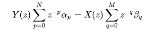
and rearranging results in

From the fundamental theorem of algebra the numerator has M roots (corresponding to zeros of H) and the denominator has N roots (corresponding to poles). Rewriting the transfer function in terms of zeros and poles

where qk is the k-th zero and pk is the k-th pole. The zeros and poles are commonly complex and when plotted on the complex plane (z-plane) it is called the pole–zero plot.
In addition, there may also exist zeros and poles at z = 0 and z = ∞. If we take these poles and zeros as well as multiple-order zeros and poles into consideration, the number of zeros and poles are always equal.
By factoring the denominator, partial fraction decomposition can be used, which can then be transformed back to the time domain. Doing so would result in the impulse response and the linear constant coefficient difference equation of the system.
If such a system H(z) is driven by a signal X(z) then the output is Y(z) = H(z)X(z). By performing partial fraction decomposition on Y(z) and then taking the inverse Z-transform the output y[n] can be found. In practice, it is often useful to fractionally decompose Y ( z ) before multiplying that quantity by z to generate a form of Y(z) which has terms with easily computable inverse Z-transforms.
by Dr. Jaydeep T. Vagh
In mathematics, the Laplace transform is an integral transform named after its inventor Pierre-Simon Laplace (/ləˈplɑːs/). It transforms a function of a real variable t (often time) to a function of a complex variable s (complex frequency). The transform has many applications in science and engineering.
The Laplace transform is similar to the Fourier transform. While the Fourier transform of a function is a complex function of a real variable (frequency), the Laplace transform of a function is a complex function of a complex variable. Laplace transforms are usually restricted to functions of t with t ≥ 0. A consequence of this restriction is that the Laplace transform of a function is a holomorphic function of the variable s. Unlike the Fourier transform, the Laplace transform of a distribution is generally a well-behaved function. Techniques of complex variables can also be used to directly study Laplace transforms. As a holomorphic function, the Laplace transform has a power series representation. This power series expresses a function as a linear superposition of moments of the function. This perspective has applications in probability theory.
The Laplace transform is invertible on a large class of functions. The inverse Laplace transform takes a function of a complex variable s (often frequency) and yields a function of a real variable t (often time). Given a simple mathematical or functional description of an input or output to a system, the Laplace transform provides an alternative functional description that often simplifies the process of analyzing the behavior of the system, or in synthesizing a new system based on a set of specifications.[1] So, for example, Laplace transformation from the time domain to the frequency domain transforms differential equations into algebraic equations and convolution into multiplication.
Laplace wrote extensively about the use of generating functions in Essai philosophique sur les probabilités (1814) and the integral form of the Laplace transform evolved naturally as a result
The Laplace transform is named after mathematician and astronomer Pierre-Simon Laplace, who used a similar transform in his work on probability theory. Laplace’s use of generating functions was similar to what is now known as the z-transform and he gave little attention to the continuous variable case which was discussed by Niels Henrik Abel. The theory was further developed in the 19th and early 20th centuries by Mathias Lerch, Oliver Heaviside, and Thomas Bromwich.[7] The current widespread use of the transform (mainly in engineering) came about during and soon after World War II replacing the earlier Heaviside operational calculus. The advantages of the Laplace transform had been emphasized by Gustav Doetsch to whom the name Laplace Transform is apparently due.
The early history of methods having some similarity to Laplace transform is as follows. From 1744, Leonhard Euler investigated integrals of the form

as solutions of differential equations but did not pursue the matter very far.
Joseph Louis Lagrange was an admirer of Euler and, in his work on integrating probability density functions, investigated expressions of the form
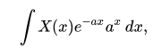
which some modern historians have interpreted within modern Laplace transform theory
These types of integrals seem first to have attracted Laplace’s attention in 1782 where he was following in the spirit of Euler in using the integrals themselves as solutions of equations.[13] However, in 1785, Laplace took the critical step forward when, rather than just looking for a solution in the form of an integral, he started to apply the transforms in the sense that was later to become popular. He used an integral of the form

akin to a Mellin transform, to transform the whole of a difference equation, in order to look for solutions of the transformed equation. He then went on to apply the Laplace transform in the same way and started to derive some of its properties, beginning to appreciate its potential power.
Laplace also recognised that Joseph Fourier’s method of Fourier series for solving the diffusion equation could only apply to a limited region of space because those solutions were periodic. In 1809, Laplace applied his transform to find solutions that diffused indefinitely in space.
The Laplace transform of a function f(t), defined for all real numbers t ≥ 0, is the function F(s), which is a unilateral transform defined by
where s is a complex number frequency parameter
An alternate notation for the Laplace transform is L instead of F.
The meaning of the integral depends on types of functions of interest. A necessary condition for existence of the integral is that f must be locally integrable on [0, ∞). For locally integrable functions that decay at infinity or are of exponential type, the integral can be understood to be a (proper) Lebesgue integral. However, for many applications it is necessary to regard it as a conditionally convergent improper integral at ∞. Still more generally, the integral can be understood in a weak sense, and this is dealt with below.
One can define the Laplace transform of a finite Borel measure μ by the Lebesgue integral

An important special case is where μ is a probability measure, for example, the Dirac delta function. In operational calculus, the Laplace transform of a measure is often treated as though the measure came from a probability density function f. In that case, to avoid potential confusion, one often writes

where the lower limit of 0− is shorthand notation for

This limit emphasizes that any point mass located at 0 is entirely captured by the Laplace transform. Although with the Lebesgue integral, it is not necessary to take such a limit, it does appear more naturally in connection with the Laplace–Stieltjes transform.
When one says “the Laplace transform” without qualification, the unilateral or one-sided transform is normally intended. The Laplace transform can be alternatively defined as the bilateral Laplace transform or two-sided Laplace transform by extending the limits of integration to be the entire real axis. If that is done the common unilateral transform simply becomes a special case of the bilateral transform where the definition of the function being transformed is multiplied by the Heaviside step function. The bilateral Laplace transform is defined as follows: F(s), which is a unilateral transform defined by

An alternate notation for the bilateral Laplace transform is B { f } instead of F.
Two integrable functions have the same Laplace transform only if they differ on a set of Lebesgue measure zero. This means that, on the range of the transform, there is an inverse transform. In fact, besides integrable functions, the Laplace transform is a one-to-one mapping from one function space into another in many other function spaces as well, although there is usually no easy characterization of the range. Typical function spaces in which this is true include the spaces of bounded continuous functions, the space L∞(0, ∞), or more generally tempered distributions on (0, ∞). The Laplace transform is also defined and injective for suitable spaces of tempered distributions.
In these cases, the image of the Laplace transform lives in a space of analytic functions in the region of convergence. The inverse Laplace transform is given by the following complex integral, which is known by various names (the Bromwich integral, the Fourier–Mellin integral, and Mellin’s inverse formula):

where γ is a real number so that the contour path of integration is in the region of convergence of F(s). An alternative formula for the inverse Laplace transform is given by Post’s inversion formula. The limit here is interpreted in the weak-* topology.
In practice, it is typically more convenient to decompose a Laplace transform into known transforms of functions obtained from a table, and construct the inverse by inspection.
In pure and applied probability, the Laplace transform is defined as an expected value. If X is a random variable with probability density function f, then the Laplace transform of f is given by the expectation
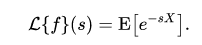
By convention, this is referred to as the Laplace transform of the random variable X itself. Replacing s by −t gives the moment generating function of X. The Laplace transform has applications throughout probability theory, including first passage times of stochastic processes such as Markov chains, and renewal theory.
Of particular use is the ability to recover the cumulative distribution function of a continuous random variable X by means of the Laplace transform as follows

If f is a locally integrable function (or more generally a Borel measure locally of bounded variation), then the Laplace transform F(s) of f converges provided that the limit

The Laplace transform converges absolutely if the integral

exists (as a proper Lebesgue integral). The Laplace transform is usually understood as conditionally convergent, meaning that it converges in the former instead of the latter sense.
The set of values for which F(s) converges absolutely is either of the form Re(s) > a or else Re(s) ≥ a, where a is an extended real constant, −∞ ≤ a ≤ ∞. (This follows from the dominated convergence theorem.) The constant a is known as the abscissa of absolute convergence, and depends on the growth behavior of f(t). Analogously, the two-sided transform converges absolutely in a strip of the form a < Re(s) < b, and possibly including the lines Re(s) = a or Re(s) = b.The subset of values of s for which the Laplace transform converges absolutely is called the region of absolute convergence or the domain of absolute convergence. In the two-sided case, it is sometimes called the strip of absolute convergence. The Laplace transform is analytic in the region of absolute convergence: this is a consequence of Fubini’s theorem and Morera’s theorem.
Similarly, the set of values for which F(s) converges (conditionally or absolutely) is known as the region of conditional convergence, or simply the region of convergence (ROC). If the Laplace transform converges (conditionally) at s = s0, then it automatically converges for all s with Re(s) > Re(s0). Therefore, the region of convergence is a half-plane of the form Re(s) > a, possibly including some points of the boundary line Re(s) = a.
In the region of convergence Re(s) > Re(s0), the Laplace transform of f can be expressed by integrating by parts as the integral
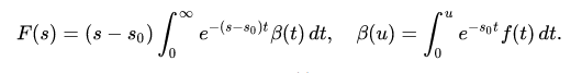
That is, in the region of convergence F(s) can effectively be expressed as the absolutely convergent Laplace transform of some other function. In particular, it is analytic.
There are several Paley–Wiener theorems concerning the relationship between the decay properties of f and the properties of the Laplace transform within the region of convergence.
In engineering applications, a function corresponding to a linear time-invariant (LTI) system is stable if every bounded input produces a bounded output. This is equivalent to the absolute convergence of the Laplace transform of the impulse response function in the region Re(s) ≥ 0. As a result, LTI systems are stable provided the poles of the Laplace transform of the impulse response function have negative real part.
This ROC is used in knowing about the causality and stability of a system.
The Laplace transform has a number of properties that make it useful for analyzing linear dynamical systems. The most significant advantage is that differentiation and integration become multiplication and division, respectively, by s (similarly to logarithms changing multiplication of numbers to addition of their logarithms).
Because of this property, the Laplace variable s is also known as operator variable in the L domain: either derivative operator or (for s−1) integration operator. The transform turns integral equations and differential equations to polynomial equations, which are much easier to solve. Once solved, use of the inverse Laplace transform reverts to the original domain.
Given the functions f(t) and g(t), and their respective Laplace transforms F(s) and G(s),
Properties of the unilateral Laplace transform

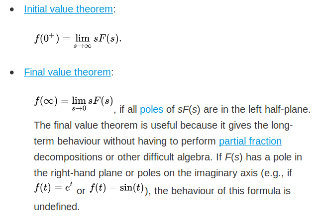
The Laplace transform can be viewed as a continuous analogue of a power series. If a(n) is a discrete function of a positive integer n, then the power series associated to a(n) is the series

where x is a real variable (see Z transform). Replacing summation over n with integration over t, a continuous version of the power series becomes
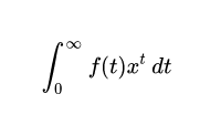
where the discrete function a(n) is replaced by the continuous one f(t).
Changing the base of the power from x to e gives

For this to converge for, say, all bounded functions f, it is necessary to require that ln x < 0. Making the substitution −s = ln x gives just the Laplace transform:
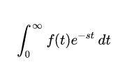
In other words, the Laplace transform is a continuous analog of a power series in which the discrete parameter n is replaced by the continuous parameter t, and x is replaced by e−s.
The quantities

are the moments of the function f. If the first n moments of f converge absolutely, then by repeated differentiation under the integral,

This is of special significance in probability theory, where the moments of a random variable X are given by the expectation values μ n = E [ X n ] . Then, the relation holds

It is often convenient to use the differentiation property of the Laplace transform to find the transform of a function’s derivative. This can be derived from the basic expression for a Laplace transform as follows:
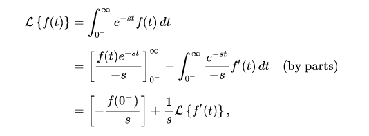
yielding

and in the bilateral case,

The general result

where f ( n )denotes the nth derivative of f, can then be established with an inductive argument.
A useful property of the Laplace transform is the following:

under suitable assumptions on the behaviour of f , g in a right neighbourhood of 0 and on the decay rate of f , g in a left neighbourhood of ∞ . The above formula is a variation of integration by parts, with the operators d d x and ∫ d x being replaced by L and L − 1
. Let us prove the equivalent formulation:

By plugging in

the left-hand side turns into:
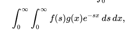
but assuming Fubini’s theorem holds, by reversing the order of integration we get the wanted right-hand side.
The (unilateral) Laplace–Stieltjes transform of a function g : R → R is defined by the Lebesgue–Stieltjes integral

The function g is assumed to be of bounded variation. If g is the antiderivative of f:

then the Laplace–Stieltjes transform of g and the Laplace transform of f coincide. In general, the Laplace–Stieltjes transform is the Laplace transform of the Stieltjes measure associated to g. So in practice, the only distinction between the two transforms is that the Laplace transform is thought of as operating on the density function of the measure, whereas the Laplace–Stieltjes transform is thought of as operating on its cumulative distribution function.
The continuous Fourier transform is equivalent to evaluating the bilateral Laplace transform with imaginary argument s = iω or s = 2πfi[24] when the condition explained below is fulfilled,

This definition of the Fourier transform requires a prefactor of 1/2 π on the reverse Fourier transform. This relationship between the Laplace and Fourier transforms is often used to determine the frequency spectrum of a signal or dynamical system.
The above relation is valid as stated if and only if the region of convergence (ROC) of F(s) contains the imaginary axis, σ = 0.
For example, the function f(t) = cos(ω0t) has a Laplace transform F(s) = s/(s2 + ω02) whose ROC is Re(s) > 0. As s = iω is a pole of F(s), substituting s = iω in F(s) does not yield the Fourier transform of f(t)u(t), which is proportional to the Dirac delta-function δ(ω − ω0).
However, a relation of the form
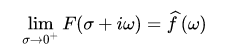
holds under much weaker conditions. For instance, this holds for the above example provided that the limit is understood as a weak limit of measures (see vague topology). General conditions relating the limit of the Laplace transform of a function on the boundary to the Fourier transform take the form of Paley–Wiener theorems.
The Mellin transform and its inverse are related to the two-sided Laplace transform by a simple change of variables.
If in the Mellin transform
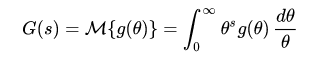
we set θ = e−t we get a two-sided Laplace transform.
The unilateral or one-sided Z-transform is simply the Laplace transform of an ideally sampled signal with the substitution of

where T = 1/fs is the sampling period (in units of time e.g., seconds) and fs is the sampling rate (in samples per second or hertz).
Let

be a sampling impulse train (also called a Dirac comb) and

be the sampled representation of the continuous-time x(t)

The Laplace transform of the sampled signal xq(t) is
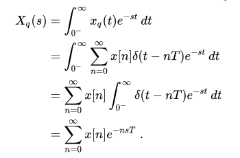
This is the precise definition of the unilateral Z-transform of the discrete function x[n]

with the substitution of z → esT.
Comparing the last two equations, we find the relationship between the unilateral Z-transform and the Laplace transform of the sampled signal,

The similarity between the Z and Laplace transforms is expanded upon in the theory of time scale calculus.
The integral form of the Borel transform

is a special case of the Laplace transform for f an entire function of exponential type, meaning that

for some constants A and B. The generalized Borel transform allows a different weighting function to be used, rather than the exponential function, to transform functions not of exponential type. Nachbin’s theorem gives necessary and sufficient conditions for the Borel transform to be well defined.
Since an ordinary Laplace transform can be written as a special case of a two-sided transform, and since the two-sided transform can be written as the sum of two one-sided transforms, the theory of the Laplace-, Fourier-, Mellin-, and Z-transforms are at bottom the same subject. However, a different point of view and different characteristic problems are associated with each of these four major integral transforms.
Table of selected Laplace transforms
The following table provides Laplace transforms for many common functions of a single variable. For definitions and explanations, see the Explanatory Notes at the end of the table.
Because the Laplace transform is a linear operator,


Using this linearity, and various trigonometric, hyperbolic, and complex number (etc.) properties and/or identities, some Laplace transforms can be obtained from others more quickly than by using the definition directly.
The unilateral Laplace transform takes as input a function whose time domain is the non-negative reals, which is why all of the time domain functions in the table below are multiples of the Heaviside step function, u(t).
The entries of the table that involve a time delay τ are required to be causal (meaning that τ > 0). A causal system is a system where the impulse response h(t) is zero for all time t prior to t = 0. In general, the region of convergence for causal systems is not the same as that of anticausal systems.


The Laplace transform is often used in circuit analysis, and simple conversions to the s-domain of circuit elements can be made. Circuit elements can be transformed into impedances, very similar to phasor impedances.
Here is a summary of equivalents:

Note that the resistor is exactly the same in the time domain and the s-domain. The sources are put in if there are initial conditions on the circuit elements. For example, if a capacitor has an initial voltage across it, or if the inductor has an initial current through it, the sources inserted in the s-domain account for that.
The equivalents for current and voltage sources are simply derived from the transformations in the table above.
by Dr. Jaydeep T. Vagh
In mathematics, the Zak transformis a certain operation which takes as input a function of one variable and produces as output a function of two variables. The output function is called the Zak transform of the input function. The transform is defined as an infinite series in which each term is a product of a dilation of a translation by an integer of the function and an exponential function. In applications of Zak transform to signal processing the input function represents a signal and the transform will be a mixed time–frequency representation of the signal. The signal may be real valued or complex-valued, defined on a continuous set (for example, the real numbers) or a discrete set (for example, the integers or a finite subset of integers). The Zak transform is a generalization of the discrete Fourier transform.
The Zak transform had been discovered by several people in different fields and was called by different names. It was called the “Gel’fand mapping” because I.M. Gel’fand introduced it in his work on eigenfunction expansions. The transform was rediscovered independently by Joshua Zak in 1967 who called it the “k-q representation”. There seems to be a general consent among experts in the field to call it the Zak transform, since Zak was the first to systematically study that transform in a more general setting and recognize its usefulness
n defining the continuous-time Zak transform, the input function is a function of a real variable. So, let f(t) be a function of a real variable t. The continuous-time Zak transform of f(t) is a function of two real variables one of which is t. The other variable may be denoted by w. The continuous-time Zak transform has been defined variously.
Let a be a positive constant. The Zak transform of f(t), denoted by Za[f], is a function of t and w defined by
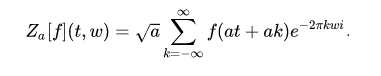
The special case of Definition 1 obtained by taking a = 1 is sometimes taken as the definition of the Zak transform.[2] In this special case, the Zak transform of f(t) is denoted by Z[f].

The notation Z[f] is used to denote another form of the Zak transform. In this form, the Zak transform of f(t) is defined as follows:
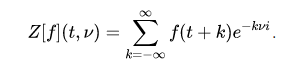
Let T be a positive constant. The Zak transform of f(t), denoted by ZT[f], is a function of t and w defined by

Here t and w are assumed to satisfy the conditions 0 ≤ t ≤ T and 0 ≤ w ≤ 1/T.
In the following it will be assumed that the Zak transform is as given in Definition 2.
Given the Zak transform of a function, the function can be reconstructed using the following formula:
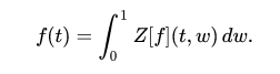
n defining the discrete Zak transform, the input function is a function of an integer variable. So, let f(n) be a function of an integer variable n (n taking all positive, zero and negative integers as values). The discrete Zak transform of f(n) is a function of two real variables one of which is the integer variable n. The other variable is a real variable which may be denoted by w. The discrete Zak transform has also been defined variously. However, only one of the definitions is given below.
The discrete Zak transform of the function f(n) where n is an integer variable, denoted by Z[f], is defined by

Given the discrete transform of a function f(n), the function can be reconstructed using the following formula:

The Zak transform has been successfully used in physics in quantum field theory, in electrical engineering in time-frequency representation of signals, and in digital data transmission. The Zak transform has also applications in mathematics. For example, it has been used in the Gabor representation problem.
by Dr. Jaydeep T. Vagh
In applied mathematics, the starred transform, or star transform, is a discrete-time variation of the Laplace transform, so-named because of the asterisk or “star” in the customary notation of the sampled signals. The transform is an operator of a continuous-time function x ( t ) , which is transformed to a function X ∗ (s) in the following manner
where δ T ( t ) is a Dirac comb function, with period of time T.
The starred transform is a convenient mathematical abstraction that represents the Laplace transform of an impulse sampled function x ∗ ( t ), which is the output of an ideal sampler, whose input is a continuous function, x ( t )
The starred transform is similar to the Z transform, with a simple change of variables, where the starred transform is explicitly declared in terms of the sampling period (T), while the Z transform is performed on a discrete signal and is independent of the sampling period. This makes the starred transform a de-normalized version of the one-sided Z-transform, as it restores the dependence on sampling parameter T.
Then per the convolution theorem, the starred transform is equivalent to the complex convolution of
hence:
This line integration is equivalent to integration in the positive sense along a closed contour formed by such a line and an infinite semicircle that encloses the poles of X(s) in the left half-plane of p. The result of such an integration (per the residue theorem) would be:
Alternatively, the aforementioned line integration is equivalent to integration in the negative sense along a closed contour formed by such a line and an infinite semicircle that encloses the infinite poles of 1 1 − e − T ( s − p ) in the right half-plane of p. The result of such an integration would be:
Given a Z-transform, X(z), the corresponding starred transform is a simple substitution:
This substitution restores the dependence on T.
It’s interchangeable
by Dr. Jaydeep T. Vagh
Post’s inversion formula for Laplace transforms, named after Emil Post,[1] is a simple-looking but usually impractical formula for evaluating an inverse Laplace transform.
The statement of the formula is as follows: Let f(t) be a continuous function on the interval [0, ∞) of exponential order, i.e.

for some real number b. Then for all s > b, the Laplace transform for f(t) exists and is infinitely differentiable with respect to s. Furthermore, if F(s) is the Laplace transform of f(t), then the inverse Laplace transform of F(s) is given by

for t > 0, where F(k) is the k-th derivative of F with respect to s.
As can be seen from the formula, the need to evaluate derivatives of arbitrarily high orders renders this formula impractical for most purposes.
With the advent of powerful personal computers, the main efforts to use this formula have come from dealing with approximations or asymptotic analysis of the Inverse Laplace transform, using the Grunwald–Letnikov differintegral to evaluate the derivatives.
Post’s inversion has attracted interest due to the improvement in computational science and the fact that it is not necessary to know where the poles of F(s) lie, which make it possible to calculate the asymptotic behaviour for big x using inverse Mellin transforms for several arithmetical functions related to the Riemann hypothesis.
by Dr. Jaydeep T. Vagh
The matched Z-transform method, also called the pole–zero mapping[1][2] or pole–zero matching method,[3] and abbreviated MPZ or MZT,[4] is a technique for converting a continuous-time filter design to a discrete-time filter (digital filter) design.
The method works by mapping all poles and zeros of the s-plane design to z-plane locations z = e s T for a sample interval T = 1 / f s So an analog filter with transfer function:
is transformed into the digital transfer function
The gain k d must be adjusted to normalize the desired gain, typically set to match the analog filter’s gain at DC by setting s = 0 z=1 and solving for k d
Since the mapping wraps the s-plane’s j ω axis around the z-plane’s unit circle repeatedly, any zeros (or poles) greater than the Nyquist frequency will be mapped to an aliased location.
In the (common) case that the analog transfer function has more poles than zeros, the zeros at s = ∞ may optionally be shifted down to the Nyquist frequency by putting them at z = − 1 z=-1, dropping off like the BLT.
This transform doesn’t preserve time- or frequency-domain response (though it does preserve stability and minimum phase), and so is not widely used.[8][7] More common methods include the bilinear transform and impulse invariance methods.[4] MZT does provide less high frequency response error than the BLT, however, making it easier to correct by adding additional zeros, which is called the MZTi (for “improved”).[9]
A specific application of the matched Z-transform method in the digital control field, is with the Ackermann’s formula, which changes the poles of the controllable system; in general from an unstable (or nearby) location to a stable location.
