by Dr. Jaydeep T. Vagh

In mathematics, an integral transform maps an equation from its original domain into another domain where it might be manipulated and solved much more easily than in the original domain. The solution is then mapped back to the original domain using the inverse of the integral transform.

General form

An integral transform is any transform T of the following form:

The input of this transform is a function f, and the output is another function Tf. An integral transform is a particular kind of mathematical operator.

There are numerous useful integral transforms. Each is specified by a choice of the function K of two variables, the kernel function, integral kernel or nucleus of the transform.

Some kernels have an associated inverse kernel K−1(u, t) which (roughly speaking) yields an inverse transform:

A symmetric kernel is one that is unchanged when the two variables are permuted; it is a kernel function K such that K(t, u) = K(u, t).

Usage example

As an example of an application of integral transforms, consider the Laplace transform. This is a technique that maps differential or integro-differential equations in the “time” domain into polynomial equations in what is termed the “complex frequency” domain. (Complex frequency is similar to actual, physical frequency but rather more general. Specifically, the imaginary component ω of the complex frequency s = -σ + iω corresponds to the usual concept of frequency, viz., the rate at which a sinusoid cycles, whereas the real component σ of the complex frequency corresponds to the degree of “damping”, i.e. an exponential decrease of the amplitude.) The equation cast in terms of complex frequency is readily solved in the complex frequency domain (roots of the polynomial equations in the complex frequency domain correspond to eigenvalues in the time domain), leading to a “solution” formulated in the frequency domain. Employing the inverse transform, i.e., the inverse procedure of the original Laplace transform, one obtains a time-domain solution. In this example, polynomials in the complex frequency domain (typically occurring in the denominator) correspond to power series in the time domain, while axial shifts in the complex frequency domain correspond to damping by decaying exponentials in the time domain.

The Laplace transform finds wide application in physics and particularly in electrical engineering, where the characteristic equations that describe the behavior of an electric circuit in the complex frequency domain correspond to linear combinations of exponentially damped, scaled, and time-shifted sinusoids in the time domain. Other integral transforms find special applicability within other scientific and mathematical disciplines.

Another usage example is the kernel in path integral:

This states that the total amplitude to arrive at ( x , t ) [that is, ψ ( x , t ) is the sum, or the integral, over all possible values of x ′ ‘ of the total amplitude to arrive at the point ( x ′ , t ′ ) multiplied by the amplitude to go from x’ to x [that is, K ( x , t ; x ′ , t ′ ) It is often referred to as the propagator of a given system. This (physics) kernel is the kernel of integral transform. However, for each quantum system, there is a different kernel.

Table of transforms

In the limits of integration for the inverse transform, c is a constant which depends on the nature of the transform function. For example, for the one and two-sided Laplace transform, c must be greater than the largest real part of the zeroes of the transform function.

Note that there are alternative notations and conventions for the Fourier transform.

Different domains

Here integral transforms are defined for functions on the real numbers, but they can be defined more generally for functions on a group.

• If instead one uses functions on the circle (periodic functions), integration kernels are then biperiodic functions; convolution by functions on the circle yields circular convolution.
• If one uses functions on the cyclic group of order n (C n or Z / nZ ), one obtains n × n matrices as integration kernels; convolution corresponds to circulant matrices.

General theory

Although the properties of integral transforms vary widely, they have some properties in common. For example, every integral transform is a linear operator, since the integral is a linear operator, and in fact if the kernel is allowed to be a generalized function then all linear operators are integral transforms (a properly formulated version of this statement is the Schwartz kernel theorem).

The general theory of such integral equations is known as Fredholm theory. In this theory, the kernel is understood to be a compact operator acting on a Banach space of functions. Depending on the situation, the kernel is then variously referred to as the Fredholm operator, the nuclear operator or the Fredholm kernel.

by Dr. Jaydeep T. Vagh

Impulse invariance is a technique for designing discrete-time infinite-impulse-response (IIR) filters from continuous-time filters in which the impulse response of the continuous-time system is sampled to produce the impulse response of the discrete-time system. The frequency response of the discrete-time system will be a sum of shifted copies of the frequency response of the continuous-time system; if the continuous-time system is approximately band-limited to a frequency less than the Nyquist frequency of the sampling, then the frequency response of the discrete-time system will be approximately equal to it for frequencies below the Nyquist frequency.

Discussion

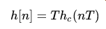
The continuous-time system’s impulse response, h c ( t ), is sampled with sampling period T to produce the discrete-time system’s impulse response, h [ n]

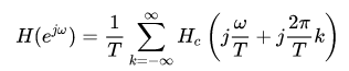
Thus, the frequency responses of the two systems are related by

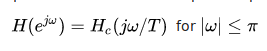
If the continuous time filter is approximately band-limited , then the frequency response of the discrete-time system will be approximately the continuous-time system’s frequency response for frequencies below π radians per sample (below the Nyquist frequency 1/(2T) Hz):

Comparison to the bilinear transform

Note that aliasing will occur, including aliasing below the Nyquist frequency to the extent that the continuous-time filter’s response is nonzero above that frequency. The bilinear transform is an alternative to impulse invariance that uses a different mapping that maps the continuous-time system’s frequency response, out to infinite frequency, into the range of frequencies up to the Nyquist frequency in the discrete-time case, as opposed to mapping frequencies linearly with circular overlap as impulse invariance does.

Poles and zeros

If the system function has zeros as well as poles, they can be mapped the same way, but the result is no longer an impulse invariance result: the discrete-time impulse response is not equal simply to samples of the continuous-time impulse response. This method is known as the matched Z-transform method, or pole–zero mapping.

Stability and causality

Since poles in the continuous-time system at s = sk transform to poles in the discrete-time system at z = exp(skT), poles in the left half of the s-plane map to inside the unit circle in the z-plane; so if the continuous-time filter is causal and stable, then the discrete-time filter will be causal and stable as well.

Effect on poles in system function

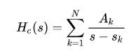
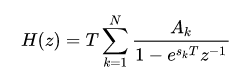
If the continuous poles at s = s k , the system function can be written in partial fraction expansion as

Thus, using the inverse Laplace transform, the impulse response is

The corresponding discrete-time system’s impulse response is then defined as the following

Performing a z-transform on the discrete-time impulse response produces the following discrete-time system function

Thus the poles from the continuous-time system function are translated to poles at z = eskT. The zeros, if any, are not so simply mapped.

Corrected formula

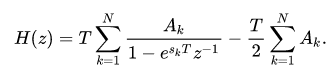
When a causal continuous-time impulse response has a discontinuity at t = 0 , the expressions above are not consistent.[1] This is because h c ( 0 )should really only contribute half its value to h [ 0 ]

Making this correction gives

Performing a z-transform on the discrete-time impulse response produces the following discrete-time system function

by Dr. Jaydeep T. Vagh

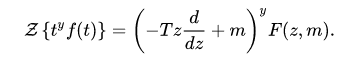
In mathematics and signal processing, the advanced z-transform is an extension of the z-transform, to incorporate ideal delays that are not multiples of the sampling time. It takes the form

where

• T is the sampling period
• m (the “delay parameter”) is a fraction of the sampling period [ 0,T.]

It is also known as the modified z-transform.

The advanced z-transform is widely applied, for example to accurately model processing delays in digital control.

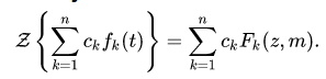
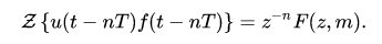
Properties

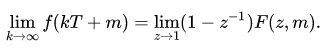
If the delay parameter, m, is considered fixed then all the properties of the z-transform hold for the advanced z-transform.

Linearity

Time shift

Damping

Time multiplication

Final value theorem

by Dr. Jaydeep T. Vagh

In mathematics and signal processing, the constant-Q transform transforms a data series to the frequency domain. It is related to the Fourier transform[1] and very closely related to the complex Morlet wavelet transform.

The transform can be thought of as a series of logarithmically spaced filters fk, with the k-th filter having a spectral width δfk equal to a multiple of the previous filter’s width:

where δf_k is the bandwidth of the k-th filter, f_min is the central frequency of the lowest filter, and n is the number of filters per octave.

Fast calculation

The direct calculation of the constant-Q transform is slow when compared against the fast Fourier transform (FFT). However, the FFT can itself be employed, in conjunction with the use of a kernel, to perform the equivalent calculation but much faster. An approximate inverse to such an implementation was proposed in 2006; it works by going back to the DFT, and is only suitable for pitch instruments.

A development on this method with improved invertibility involves performing CQT (via FFT) octave-by-octave, using lowpass filtered and downsampled results for consecutively lower pitches.[5] Implementations of this method include the reference MATLAB implementation and LibROSA’s Python implementation.LibROSA combines the subsampled method with the direct FFT method (which it dubs “pseudo-CQT”) by having the latter process higher frequencies as a whole.

Comparison with the Fourier transform

In general, the transform is well suited to musical data, and this can be seen in some of its advantages compared to the fast Fourier transform. As the output of the transform is effectively amplitude/phase against log frequency, fewer frequency bins are required to cover a given range effectively, and this proves useful where frequencies span several octaves. As the range of human hearing covers approximately ten octaves from 20 Hz to around 20 kHz, this reduction in output data is significant.

The transform exhibits a reduction in frequency resolution with higher frequency bins, which is desirable for auditory applications. The transform mirrors the human auditory system, whereby at lower-frequencies spectral resolution is better, whereas temporal resolution improves at higher frequencies. At the bottom of the piano scale (about 30 Hz), a difference of 1 semitone is a difference of approximately 1.5 Hz, whereas at the top of the musical scale (about 5 kHz), a difference of 1 semitone is a difference of approximately 200 Hz. So for musical data the exponential frequency resolution of constant-Q transform is ideal.

In addition, the harmonics of musical notes form a pattern characteristic of the timbre of the instrument in this transform. Assuming the same relative strengths of each harmonic, as the fundamental frequency changes, the relative position of these harmonics remains constant. This can make identification of instruments much easier. The constant Q transform can also be used for automatic recognition of musical keys based on accumulated chroma content.

Relative to the Fourier transform, implementation of this transform is more tricky. This is due to the varying number of samples used in the calculation of each frequency bin, which also affects the length of any windowing function implemented.

Also note that because the frequency scale is logarithmic, there is no true zero-frequency / DC term present, perhaps limiting possible utility of the transform.

by Dr. Jaydeep T. Vagh

In mathematics, the discrete-time Fourier transform (DTFT) is a form of Fourier analysis that is applicable to a sequence of values.

The DTFT is often used to analyze samples of a continuous function. The term discrete-time refers to the fact that the transform operates on discrete data, often samples whose interval has units of time. From uniformly spaced samples it produces a function of frequency that is a periodic summation of the continuous Fourier transform of the original continuous function. Under certain theoretical conditions, described by the sampling theorem, the original continuous function can be recovered perfectly from the DTFT and thus from the original discrete samples. The DTFT itself is a continuous function of frequency, but discrete samples of it can be readily calculated via the discrete Fourier transform (DFT) (see Sampling the DTFT), which is by far the most common method of modern Fourier analysis.

Both transforms are invertible. The inverse DTFT is the original sampled data sequence. The inverse DFT is a periodic summation of the original sequence. The fast Fourier transform (FFT) is an algorithm for computing one cycle of the DFT, and its inverse produces one cycle of the inverse DFT.

Definition

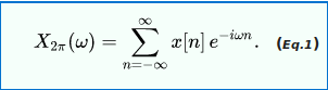
The discrete-time Fourier transform of a discrete set of real or complex numbers x[n], for all integers n, is a Fourier series, which produces a periodic function of a frequency variable. When the frequency variable, ω, has normalized units of radians/sample, the periodicity is 2π, and the Fourier series is:

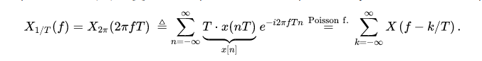
The utility of this frequency domain function is rooted in the Poisson summation formula. Let X(f) be the Fourier transform of any function, x(t), whose samples at some interval T (seconds) are equal (or proportional) to the x[n] sequence, i.e. T⋅x(nT) = x[n]. Then the periodic function represented by the Fourier series is a periodic summation of X(f) in terms of frequency f in hertz (cycles/sec):

The integer k has units of cycles/sample, and 1/T is the sample-rate, fs (samples/sec). So X1/T(f) comprises exact copies of X(f) that are shifted by multiples of fs hertz and combined by addition. For sufficiently large fs the k = 0 term can be observed in the region [−fs/2, fs/2] with little or no distortion (aliasing) from the other terms. In Fig.1, the extremities of the distribution in the upper left corner are masked by aliasing in the periodic summation (lower left).

We also note that e−i2πfTn is the Fourier transform of δ(t − nT). Therefore, an alternative definition of DTFT is:

The modulated Dirac comb function is a mathematical abstraction sometimes referred to as impulse sampling.

Inverse transform

An operation that recovers the discrete data sequence from the DTFT function is called an inverse DTFT. For instance, the inverse continuous Fourier transform of both sides of Eq.3 produces the sequence in the form of a modulated Dirac comb function:

However, noting that X1/T(f) is periodic, all the necessary information is contained within any interval of length 1/T. In both Eq.1 and Eq.2, the summations over n are a Fourier series, with coefficients x[n]. The standard formulas for the Fourier coefficients are also the inverse transforms:

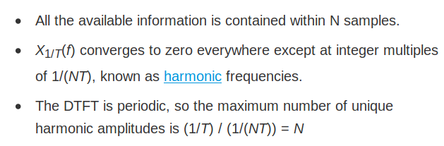
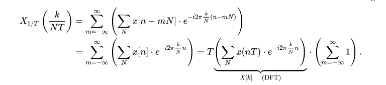
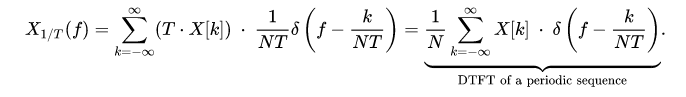
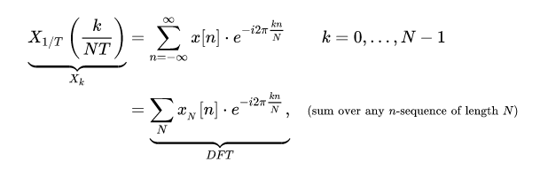
Periodic data

When the input data sequence x[n] is N-periodic, Eq.2 can be computationally reduced to a discrete Fourier transform (DFT), because:

Therefore, the DTFT diverges at the harmonic frequencies, but at different frequency-dependent rates. And those rates are given by the DFT of one cycle of the x[n] sequence. In terms of a Dirac comb function, this is represented by:

Sampling the DTFT

When the DTFT is continuous, a common practice is to compute an arbitrary number of samples (N) of one cycle of the periodic function X1/T:

where is a periodic summation:

The N sequence is the inverse DFT. Thus, our sampling of the DTFT causes the inverse transform to become periodic. The array of |Xk|2 values is known as a periodogram, and the parameter N is called NFFT in the Matlab function of the same name.

In order to evaluate one cycle of numerically, we require a finite-length x[n] sequence. For instance, a long sequence might be truncated by a window function of length L resulting in three cases worthy of special mention. For notational simplicity, consider the x[n] values below to represent the values modified by the window function.

Case: Frequency decimation. L = N ⋅ I, for some integer I (typically 6 or 8)

A cycle of x N reduces to a summation of I blocks of length N, or circular addition. The DFT then goes by various names, such as:

• window-presum FFT
• Weight, overlap, add (WOLA)
• polyphase FFT
• polyphase filter bank
• multiple block windowing and time-aliasing.

Recall that decimation of sampled data in one domain (time or frequency) produces overlap (sometimes known as aliasing) in the other, and vice versa. Compared to an L-length DFT, the xN summation/overlap causes decimation in frequency, leaving only DTFT samples least affected by spectral leakage. That is usually a priority when implementing an FFT filter-bank (channelizer). With a conventional window function of length L, scalloping loss would be unacceptable. So multi-block windows are created using FIR filter design tools. Their frequency profile is flat at the highest point and falls off quickly at the midpoint between the remaining DTFT samples. The larger the value of parameter I, the better the potential performance.

Case: L = N+1, where N is even-valued

This case arises in the context of Window function design, out of a desire for real-valued DFT coefficients. When a symmetric sequence is associated with the indices [-M ≤ n ≤ M], known as a finite Fourier transform data window, its DTFT, a continuous function of frequency f(n) is real-valued. When the sequence is shifted into a DFT data window, [0 ≤ n ≤ 2M], the DTFT is multiplied by a complex-valued phase function: e − i2πfMBut when sampled at frequencies f=k / 2M for integer values of k he samples are all real-valued. To achieve that goal, we can perform a 2 -length DFT on a periodic summation with 1-sample of overlap. Specifically, the last sample of a data sequence is deleted and its value added to the first sample. Then a window function, shortened by 1 sample, is applied, and the DFT is performed. The shortened, even-length window function is sometimes called DFT-even. In actual practice, people commonly use DFT-even windows without overlapping the data, because the detrimental effects on spectral leakage are negligible for long sequences (typically hundreds of samples).

Convolution

The convolution theorem for sequences is:

An important special case is the circular convolution of sequences x and y defined by x N ∗ y where x N is a periodic summation. The discrete-frequency nature of DTFT{xN} “selects” only discrete values from the continuous function DTFT{y}, which results in considerable simplification of the inverse transform. As shown at Convolution theorem#Functions of discrete variable sequences:

For x and y sequences whose non-zero duration is less than or equal to N, a final simplification is:

The significance of this result is expounded at Circular convolution and Fast convolution algorithms.

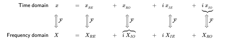
Symmetry properties

When the real and imaginary parts of a complex function are decomposed into their even and odd parts, there are four components, denoted below by the subscripts RE, RO, IE, and IO. And there is a one-to-one mapping between the four components of a complex time function and the four components of its complex frequency transform

From this, various relationships are apparent, for example:

Relationship to the Z-transform

X 2 π ( ω ) is a Fourier series that can also be expressed in terms of the bilateral Z-transform. I.e.:

where the X ^ notation distinguishes the Z-transform from the Fourier transform. Therefore, we can also express a portion of the Z-transform in terms of the Fourier transform:

Note that when parameter T changes, the terms of X 2 π ( ω ) remain a constant separation 2 π apart, and their width scales up or down. The terms of X1/T(f) remain a constant width and their separation 1/T scales up or down.

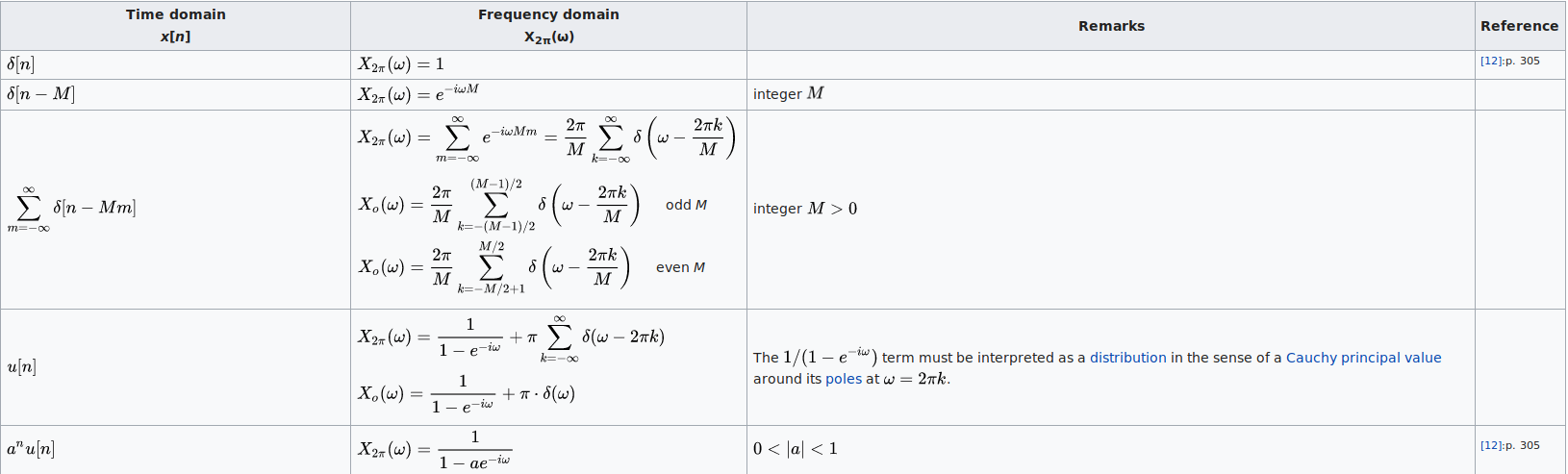
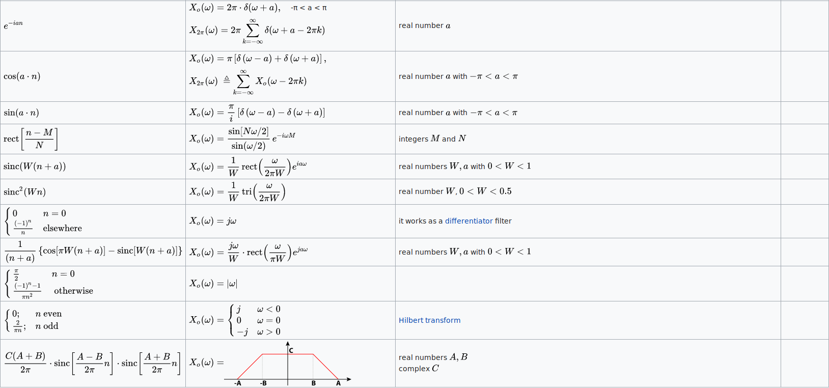
Table of discrete-time Fourier transforms

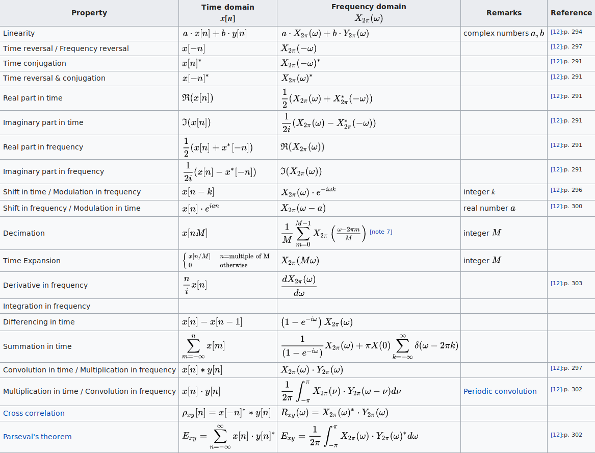
Properties

This table shows some mathematical operations in the time domain and the corresponding effects in the frequency domain.

by Dr. Jaydeep T. Vagh

That mathematical knowledge only parpose in Signal processing

In mathematics, the discrete Fourier transform (DFT) converts a finite sequence of equally-spaced samples of a function into a same-length sequence of equally-spaced samples of the discrete-time Fourier transform (DTFT), which is a complex-valued function of frequency. The interval at which the DTFT is sampled is the reciprocal of the duration of the input sequence. An inverse DFT is a Fourier series, using the DTFT samples as coefficients of complex sinusoids at the corresponding DTFT frequencies. It has the same sample-values as the original input sequence. The DFT is therefore said to be a frequency domain representation of the original input sequence. If the original sequence spans all the non-zero values of a function, its DTFT is continuous (and periodic), and the DFT provides discrete samples of one cycle. If the original sequence is one cycle of a periodic function, the DFT provides all the non-zero values of one DTFT cycle

The DFT is the most important discrete transform, used to perform Fourier analysis in many practical applications.[1] In digital signal processing, the function is any quantity or signal that varies over time, such as the pressure of a sound wave, a radio signal, or daily temperature readings, sampled over a finite time interval (often defined by a window function[2]). In image processing, the samples can be the values of pixels along a row or column of a raster image. The DFT is also used to efficiently solve partial differential equations, and to perform other operations such as convolutions or multiplying large integers.

Since it deals with a finite amount of data, it can be implemented in computers by numerical algorithms or even dedicated hardware. These implementations usually employ efficient fast Fourier transform (FFT) algorithms;[3] so much so that the terms “FFT” and “DFT” are often used interchangeably. Prior to its current usage, the “FFT” initialism may have also been used for the ambiguous term “finite Fourier transform”.

Definition

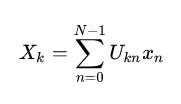
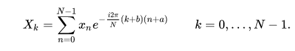
The discrete Fourier transform transforms a sequence of N complex numbers { x n } := x 0 , x 1 , … , x N − 1 into another sequence of complex numbers, { X k } := X 0 , X 1 , … , X N − 1 , which is defined by

where the last expression follows from the first one by Euler’s formula.

The transform is sometimes denoted by the symbol

Motivation

Eq.1 can also be evaluated outside the domain

and that extended sequence is N N-periodic. Accordingly, other sequences of N indices are sometimes used, such as

(if N N is even) and

which amounts to swapping the left and right halves of the result of the transform.

Eq.1 can be interpreted or derived in various ways, for example:

• It completely describes the discrete-time Fourier transform (DTFT) of an N -periodic sequence, which comprises only discrete frequency components. (Using the DTFT with periodic data)
• It can also provide uniformly spaced samples of the continuous DTFT of a finite length sequence. (Sampling the DTFT)
• It is the cross correlation of the input sequence, x n, and a complex sinusoid at frequency k/ N .  Thus it acts like a matched filter for that frequency.
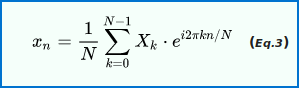
• It is the discrete analog of the formula for the coefficients of a Fourier series:

which is also NN-periodic. In the domain n ∈ [0, N − 1], this is the inverse transform of Eq.1. In this interpretation, each X is a complex number that encodes both amplitude and phase of a complex sinusoidal component ( e i 2 π k n / N )

of function x n .The sinusoid’s frequency is k cycles per N samples. Its amplitude and phase are:

where atan2 is the two-argument form of the arctan function. In polar form

here cis is the mnemonic for cos + i sin.

The normalization factor multiplying the DFT and IDFT (here 1 and 1/N) and the signs of the exponents are merely conventions, and differ in some treatments. The only requirements of these conventions are that the DFT and IDFT have opposite-sign exponents and that the product of their normalization factors be 1 / N 1/N. A normalization of 1 / N for both the DFT and IDFT, for instance, makes the transforms unitary. A discrete impulse, x n = 1 at n = 0 and 0 otherwise; might transform to X k = 1 for all k (use normalization factors 1 for DFT and 1/N for IDFT). A DC signal, X k = 1 at k = 0 and 0 otherwise; might inversely transform to x n = 1 for all n 1/N for DFT and 1 for IDFT) which is consistent with viewing DC as the mean average of the signal.

Inverse transform

The discrete Fourier transform is an invertible, linear transformation

with C denoting the set of complex numbers. This is known as Inverse Discrete Fourier Transform(IDFT). In other words, for any N > 0 N>0, an N-dimensional complex vector has a DFT and an IDFT which are in turn N N-dimensional complex vectors.

The inverse transform is given by:

Properties

Linearity

The DFT is a linear transform

then for any complex numbers a,b:

Time and frequency reversal

Reversing the time in x n to reversing the frequency Mathematically, if { x n } represents the vector x then Reversing the time in x n to reversing the frequency

Conjugation in time

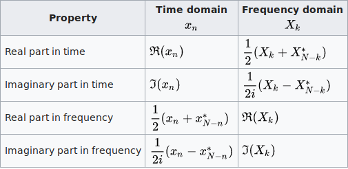
Real and imaginary part

This table shows some mathematical operations on x n in the time domain and the corresponding effects on its DFT X k in the frequency domain.

Orthogonality

where δ k k ′ is the Kronecker delta. (In the last step, the summation is trivial if k = k ′ k=k’, where it is 1+1+⋅⋅⋅=N, and otherwise is a geometric series that can be explicitly summed to obtain zero.) This orthogonality condition can be used to derive the formula for the IDFT from the definition of the DFT, and is equivalent to the unitarity property below.

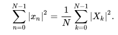
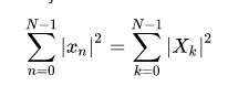
The Plancherel theorem and Parseval’s theorem

If X k the DFTs of x n respectively then the Parseval’s theorem states:

where the star denotes complex conjugation. Plancherel theorem is a special case of the Parseval’s theorem and states:

These theorems are also equivalent to the unitary condition below.

Periodicity

The periodicity can be shown directly from the definition:

Similarly, it can be shown that the IDFT formula leads to a periodic extension.

Shift theorem

Circular convolution theorem and cross-correlation theorem

The convolution theorem for the discrete-time Fourier transform indicates that a convolution of two infinite sequences can be obtained as the inverse transform of the product of the individual transforms. An important simplification occurs when the sequences are of finite length, N. In terms of the DFT and inverse DFT, it can be written as follows:

which is the convolution of the x sequence with a y sequence extended by periodic summation:

Similarly, the cross-correlation of x and y N is given by:

When either sequence contains a string of zeros, of length L L+1 of the circular convolution outputs are equivalent to values of x ∗ y . . Methods have also been developed to use this property as part of an efficient process that constructs x ∗ y with an x or y sequence potentially much longer than the practical transform size ( N N). Two such methods are called overlap-save and overlap-add.[6] The efficiency results from the fact that a direct evaluation of either summation (above) requires O ( N 2 ) ) operations for an output sequence of length N N. An indirect method, using transforms, can take advantage of the O ( N log ⁡ N ) \scriptstyle O(N\log N) efficiency of the fast Fourier transform (FFT) to achieve much better performance. Furthermore, convolutions can be used to efficiently compute DFTs via Rader’s FFT algorithm and Bluestein’s FFT algorithm.

Convolution theorem duality

It can also be shown that:

Trigonometric interpolation polynomial

The trigonometric interpolation polynomial

where the coefficients Xk are given by the DFT of xn above, satisfies the interpolation property p ( n / N ) = x n for n = 0 , … , N − 1 n=0,\ldots ,N-1.

For even N, notice that the Nyquist component

is handled specially.

This interpolation is not unique: aliasing implies that one could add N to any of the complex-sinusoid frequencies (e.g. changing e − i t ) without changing the interpolation property, but giving different values in between the x n points. The choice above, however, is typical because it has two useful properties. First, it consists of sinusoids whose frequencies have the smallest possible magnitudes: the interpolation is bandlimited. Second, if the x n are real numbers, then p ( t ) p(t) is real as well.

In contrast, the most obvious trigonometric interpolation polynomial is the one in which the frequencies range from 0 to N − 1 N-1 (instead of roughly − N / 2 -N/2 to + N / 2 +N/2 as above), similar to the inverse DFT formula. This interpolation does not minimize the slope, and is not generally real-valued for real x n its use is a common mistake.

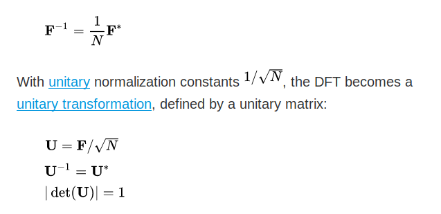
The unitary DFT

Another way of looking at the DFT is to note that in the above discussion, the DFT can be expressed as the DFT matrix, a Vandermonde matrix, introduced by Sylvester in 1867,

The inverse transform is then given by the inverse of the above matrix,

where det is the determinant function. The determinant is the product of the eigenvalues, which are always \pm 1 or \pm i as described below. In a real vector space, a unitary transformation can be thought of as simply a rigid rotation of the coordinate system, and all of the properties of a rigid rotation can be found in the unitary DFT.

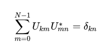
The orthogonality of the DFT is now expressed as an orthonormality condition (which arises in many areas of mathematics as described in root of unity):

If X is defined as the unitary DFT of the vector x, then

and the Plancherel theorem is expressed as

If we view the DFT as just a coordinate transformation which simply specifies the components of a vector in a new coordinate system, then the above is just the statement that the dot product of two vectors is preserved under a unitary DFT transformation. For the special case x = y , this implies that the length of a vector is preserved as well—this is just Parseval’s theorem,

A consequence of the circular convolution theorem is that the DFT matrix F diagonalizes any circulant matrix.

Expressing the inverse DFT in terms of the DFT

A useful property of the DFT is that the inverse DFT can be easily expressed in terms of the (forward) DFT, via several well-known “tricks”. (For example, in computations, it is often convenient to only implement a fast Fourier transform corresponding to one transform direction and then to get the other transform direction from the first.)

First, we can compute the inverse DFT by reversing all but one of the inputs (Duhamel et al., 1988):

(As usual, the subscripts are interpreted modulo N; thus, for n = 0 n=0, we have x N − 0 = x 0

Second, one can also conjugate the inputs and outputs:

Third, a variant of this conjugation trick, which is sometimes preferable because it requires no modification of the data values, involves swapping real and imaginary parts (which can be done on a computer simply by modifying pointers). Define swap ⁡ ( x n ) ) ) as x n with its real and imaginary parts swapped—that is, if x n = a + b i x_{n}=a+bi then swap ⁡ ( x n ) is b + a i b+ai. Equivalently, swap ⁡ ( x n ) \operatorname ) equals i x n ∗ . Then

That is, the inverse transform is the same as the forward transform with the real and imaginary parts swapped for both input and output, up to a normalization (Duhamel et al., 1988).

The conjugation trick can also be used to define a new transform, closely related to the DFT, that is involutory—that is, which is its own inverse. In particular T is clearly its ownThe conjugation trick can also be used to define a new transform, closely related to the DFT, that is involutory—that is, which is its own inverse. In particular

Eigenvalues and eigenvectors

The eigenvalues of the DFT matrix are simple and well-known, whereas the eigenvectors are complicated, not unique, and are the subject of ongoing research.

Consider the unitary form U defined above for the DFT of length N, where

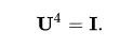
This matrix satisfies the matrix polynomial equation:

This can be seen from the inverse properties above: operating U twice gives the original data in reverse order, so operating U four times gives back the original data and is thus the identity matrix. This means that the eigenvalues λ lambda satisfy the equation:

Therefore, the eigenvalues of U \lambda is +1, −1, +i, or −i.

Since there are only four distinct eigenvalues for this N × N {\displaystyle N\times N} N\times N matrix, they have some multiplicity. The multiplicity gives the number of linearly independent eigenvectors corresponding to each eigenvalue. (There are N independent eigenvectors; a unitary matrix is never defective.)

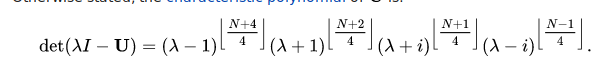
The problem of their multiplicity was solved by McClellan and Parks (1972), although it was later shown to have been equivalent to a problem solved by Gauss (Dickinson and Steiglitz, 1982). The multiplicity depends on the value of N modulo 4, and is given by the following table:

Otherwise stated, the characteristic polynomial of U is:

No simple analytical formula for general eigenvectors is known. Moreover, the eigenvectors are not unique because any linear combination of eigenvectors for the same eigenvalue is also an eigenvector for that eigenvalue. Various researchers have proposed different choices of eigenvectors, selected to satisfy useful properties like orthogonality and to have “simple” forms (e.g., McClellan and Parks, 1972; Dickinson and Steiglitz, 1982; Grünbaum, 1982; Atakishiyev and Wolf, 1997; Candan et al., 2000; Hanna et al., 2004; Gurevich and Hadani, 2008).

A straightforward approach is to discretize an eigenfunction of the continuous Fourier transform, of which the most famous is the Gaussian function. Since periodic summation of the function means discretizing its frequency spectrum and discretization means periodic summation of the spectrum, the discretized and periodically summed Gaussian function yields an eigenvector of the discrete transform:

The closed form expression for the series can be expressed by Jacobi theta functions as

Two other simple closed-form analytical eigenvectors for special DFT period N were found (Kong, 2008):

For DFT period N = 2L + 1 = 4K + 1, where K is an integer, the following is an eigenvector of DFT:

The choice of eigenvectors of the DFT matrix has become important in recent years in order to define a discrete analogue of the fractional Fourier transform—the DFT matrix can be taken to fractional powers by exponentiating the eigenvalues (e.g., Rubio and Santhanam, 2005). For the continuous Fourier transform, the natural orthogonal eigenfunctions are the Hermite functions, so various discrete analogues of these have been employed as the eigenvectors of the DFT, such as the Kravchuk polynomials (Atakishiyev and Wolf, 1997). The “best” choice of eigenvectors to define a fractional discrete Fourier transform remains an open question, however.

Uncertainty principles

Probabilistic uncertainty principle

If the random variable Xk is constrained by

then

may be considered to represent a discrete probability mass function of n, with an associated probability mass function constructed from the transformed variable,

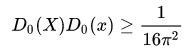
For the case of continuous functions P ( x ) Q(k), the Heisenberg uncertainty principle states that

where D 0 ( X ) (x) are the variances of | X | 2 respectively, with the equality attained in the case of a suitably normalized Gaussian distribution. Although the variances may be analogously defined for the DFT, an analogous uncertainty principle is not useful, because the uncertainty will not be shift-invariant. Still, a meaningful uncertainty principle has been introduced by Massar and Spindel.

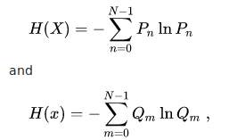
However, the Hirschman entropic uncertainty will have a useful analog for the case of the DFT. The Hirschman uncertainty principle is expressed in terms of the Shannon entropy of the two probability functions.

In the discrete case, the Shannon entropies are defined as

and the entropic uncertainty principle becomes

The equality is obtained for P nequal to translations and modulations of a suitably normalized Kronecker comb of period A A where A is any exact integer divisor of N. The probability mass function Q mwill then be proportional to a suitably translated Kronecker comb of period B = N / A

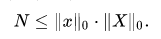
Deterministic uncertainty principle

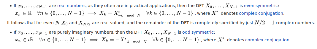
DFT of real and purely imaginary signals

Generalized DFT (shifted and non-linear phase)

is possible to shift the transform sampling in time and/or frequency domain by some real shifts a and b, respectively. This is sometimes known as a generalized DFT (or GDFT), also called the shifted DFT or offset DFT, and has analogous properties to the ordinary DFT:

Most often, shifts of 1 / 2 (half a sample) are used. While the ordinary DFT corresponds to a periodic signal in both time and frequency domains, a = 1 / 2produces a signal that is anti-periodic in frequency domain. Such shifted transforms are most often used for symmetric data, to represent different boundary symmetries, and for real-symmetric data they correspond to different forms of the discrete cosine and sine transforms.

Another interesting choice is a = b = − ( N − 1 ) / 2 a=b=-(N-1)/2, which is called the centered DFT (or CDFT). The centered DFT has the useful property that, when N is a multiple of four, all four of its eigenvalues (see above) have equal multiplicities (Rubio and Santhanam, 2005)

The term GDFT is also used for the non-linear phase extensions of DFT. Hence, GDFT method provides a generalization for constant amplitude orthogonal block transforms including linear and non-linear phase types. GDFT is a framework to improve time and frequency domain properties of the traditional DFT, e.g. auto/cross-correlations, by the addition of the properly designed phase shaping function (non-linear, in general) to the original linear phase functions (Akansu and Agirman-Tosun, 2010).

The discrete Fourier transform can be viewed as a special case of the z-transform, evaluated on the unit circle in the complex plane; more general z-transforms correspond to complex shifts a and b above.

Multidimensional DFT

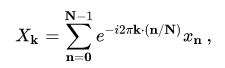
The ordinary DFT transforms a one-dimensional sequence or array x n that is a function of exactly one discrete variable n. The multidimensional DFT of a multidimensional array x n 1 , n 2 , … , n d that is a function of d discrete variables n ℓ = 0 , 1 , … , N ℓ − 1 ,d is defined by:

where ω N ℓ = exp ⁡ ( − i 2 π / N ℓ ) as above and the d output indices run from k ℓ = 0 , 1 , … , N ℓ -1. This is more compactly expressed in vector notation, where we define n = ( n 1 , n 2 , … , n d ) and k = ( k 1 , k 2 , … , k d ) as d-dimensional vectors of indices from 0 to N − 1 , which we define as N − 1 = ( N 1 − 1 , N 2 − 1 , … , N d − 1 )

where the division n / N is defined as n / N = ( n 1 / N 1 , … , n d / N d ) to be performed element-wise, and the sum denotes the set of nested summations above.

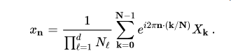
The inverse of the multi-dimensional DFT is, analogous to the one-dimensional case, given by:

As the one-dimensional DFT expresses the input x n as a superposition of sinusoids, the multidimensional DFT expresses the input as a superposition of plane waves, or multidimensional sinusoids. The direction of oscillation in space is k / N . This decomposition is of great importance for everything from digital image processing (two-dimensional) to solving partial differential equations. The solution is broken up into plane waves.

The multidimensional DFT can be computed by the composition of a sequence of one-dimensional DFTs along each dimension. In the two-dimensional case x n 1 , n 2 independent DFTs of the rows (i.e., along n 2) are computed first to form a new array y n 1 , k 2 . Then the N 2 independent DFTs of y along the columns (along n 1 are computed to form the final result X k 1 , k 2 . Alternatively the columns can be computed first and then the rows. The order is immaterial because the nested summations above commute.

An algorithm to compute a one-dimensional DFT is thus sufficient to efficiently compute a multidimensional DFT. This approach is known as the row-column algorithm. There are also intrinsically multidimensional FFT algorithms.

The real-input multidimensional DFT

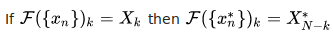
For input data x n 1 , n 2 , … , n d consisting of real numbers, the DFT outputs have a conjugate symmetry similar to the one-dimensional case above:

where the star again denotes complex conjugation and the ℓell -th subscript is again interpreted modulo N

Some discrete Fourier transform pairs

by Dr. Jaydeep T. Vagh

Discrete-time approximation

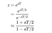
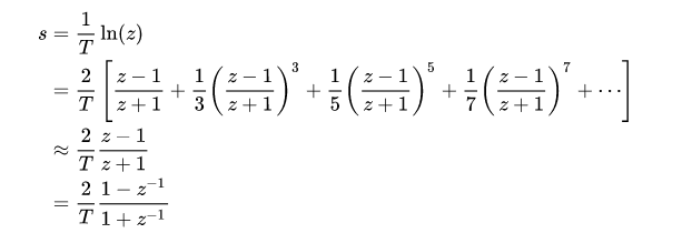
The bilinear transform is a first-order approximation of the natural logarithm function that is an exact mapping of the z-plane to the s-plane. When the Laplace transform is performed on a discrete-time signal (with each element of the discrete-time sequence attached to a correspondingly delayed unit impulse), the result is precisely the Z transform of the discrete-time sequence with the substitution of

where T is the numerical integration step size of the trapezoidal rule used in the bilinear transform derivation; or, in other words, the sampling period. The above bilinear approximation can be solved for s or a similar approximation for s=(1/T)\ln(z) can be performed.

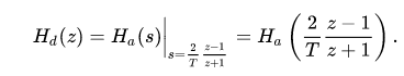
The bilinear transform essentially uses this first order approximation and substitutes into the continuous-time transfer function, Ha (s)

That is

Stability and minimum-phase property preserved

A continuous-time causal filter is stable if the poles of its transfer function fall in the left half of the complex s-plane. A discrete-time causal filter is stable if the poles of its transfer function fall inside the unit circle in the complex z-plane. The bilinear transform maps the left half of the complex s-plane to the interior of the unit circle in the z-plane. Thus, filters designed in the continuous-time domain that are stable are converted to filters in the discrete-time domain that preserve that stability.

Likewise, a continuous-time filter is minimum-phase if the zeros of its transfer function fall in the left half of the complex s-plane. A discrete-time filter is minimum-phase if the zeros of its transfer function fall inside the unit circle in the complex z-plane. Then the same mapping property assures that continuous-time filters that are minimum-phase are converted to discrete-time filters that preserve that property of being minimum-phase.

Example

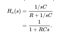
As an example take a simple low-passRC filter. This continuous-time filter has a transfer function

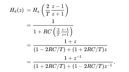
If we wish to implement this filter as a digital filter, we can apply the bilinear transform by substituting for s the formula above; after some reworking, we get the following filter representation:

The coefficients of the denominator are the ‘feed-backward’ coefficients and the coefficients of the numerator are the ‘feed-forward’ coefficients used to implement a real-time digital filter.

Transformation for a general first-order continuous-time filter

It is possible to relate the coefficients of a continuous-time, analog filter with those of a similar discrete-time digital filter created through the bilinear transform process. Transforming a general, first-order continuous-time filter with the given transfer function

using the bilinear transform (without prewarping any frequency specification) requires the substitution of

where

However, if the frequency warping compensation as described below is used in the bilinear transform, so that both analog and digital filter gain and phase agree at frequency ω 0, then

This results in a discrete-time digital filter with coefficients expressed in terms of the coefficients of the original continuous time filter:

Normally the constant term in the denominator must be normalized to 1 before deriving the corresponding difference equation. This results in

The difference equation (using the Direct Form I) is

General second-order biquad transformation

A similar process can be used for a general second-order filter with the given transfer function

This results in a discrete-time digital biquad filter with coefficients expressed in terms of the coefficients of the original continuous time filter:

Again, the constant term in the denominator is generally normalized to 1 before deriving the corresponding difference equation. This results in

The difference equation (using the Direct Form I) is

Frequency warping

o determine the frequency response of a continuous-time filter, the transfer function H a ( s ) is evaluated at s = j ω a which is on the j ω axis. Likewise, to determine the frequency response of a discrete-time filter, the transfer function H d ( z ) is evaluated at z = e j ω d T which is on the unit circle, | z | = 1 . The bilinear transform maps the j ω axis of the s-plane (of which is the domain of H a ( s ) to the unit circle of the z-plane, | z | = 1 (which is the domain of H d ( z ) , but it is not the same mapping z = e s T which also maps the j ωaxis to the unit circle. When the actual frequency of ω d is input to the discrete-time filter designed by use of the bilinear transform, then it is desired to know at what frequency, ω a, for the continuous-time filter that this ω d is mapped to.

This shows that every point on the unit circle in the discrete-time filter z-plane, z = e j ω d T is mapped to a point on the j ω j omega axis on the continuous-time filter s-plane, s = j ω a . That is, the discrete-time to continuous-time frequency mapping of the bilinear transform is

and the inverse mapping is

The discrete-time filter behaves at frequency ω d the same way that the continuous-time filter behaves at frequency ( 2 / T ) tan ⁡ ( ω d T / 2 ) . Specifically, the gain and phase shift that the discrete-time filter has at frequency ω d is the same gain and phase shift that the continuous-time filter has at frequency ( 2 / T ) tan ⁡ ( ω d T / 2 ) . This means that every feature, every “bump” that is visible in the frequency response of the continuous-time filter is also visible in the discrete-time filter, but at a different frequency. For low frequencies (that is, when ω d ≪ 2 / T or ω a ≪ 2 / T, then the features are mapped to a slightly different frequency; ω d ≈ ω a

One can see that the entire continuous frequency range

is mapped onto the fundamental frequency interval

The continuous-time filter frequency ω a = 0 corresponds to the discrete-time filter frequency ω d = 0 and the continuous-time filter frequency ω a = ± ∞ correspond to the discrete-time filter frequency ω d = ± π / T .

One can also see that there is a nonlinear relationship between ω a and ω d . This effect of the bilinear transform is called frequency warping. The continuous-time filter can be designed to compensate for this frequency warping by setting

for every frequency specification that the designer has control over (such as corner frequency or center frequency). This is called pre-warping the filter design.

It is possible, however, to compensate for the frequency warping by pre-warping a frequency specification ω 0(usually a resonant frequency or the frequency of the most significant feature of the frequency response) of the continuous-time system. These pre-warped specifications may then be used in the bilinear transform to obtain the desired discrete-time system. When designing a digital filter as an approximation of a continuous time filter, the frequency response (both amplitude and phase) of the digital filter can be made to match the frequency response of the continuous filter at a specified frequency ω 0, as well as matching at DC, if the following transform is substituted into the continuous filter transfer function.[2] This is a modified version of Tustin’s transform shown above

However, note that this transform becomes the original transform

The main advantage of the warping phenomenon is the absence of aliasing distortion of the frequency response characteristic, such as observed with Impulse invariance.

by Dr. Jaydeep T. Vagh

In signal processing, sampling is the reduction of a continuous-time signal to a discrete-time signal. A common example is the conversion of a sound wave (a continuous signal) to a sequence of samples (a discrete-time signal).

A sample is a value or set of values at a point in time and/or space.

A sampler is a subsystem or operation that extracts samples from a continuous signal.

A theoretical ideal sampler produces samples equivalent to the instantaneous value of the continuous signal at the desired points.

Theory

Sampling can be done for functions varying in space, time, or any other dimension, and similar results are obtained in two or more dimensions.

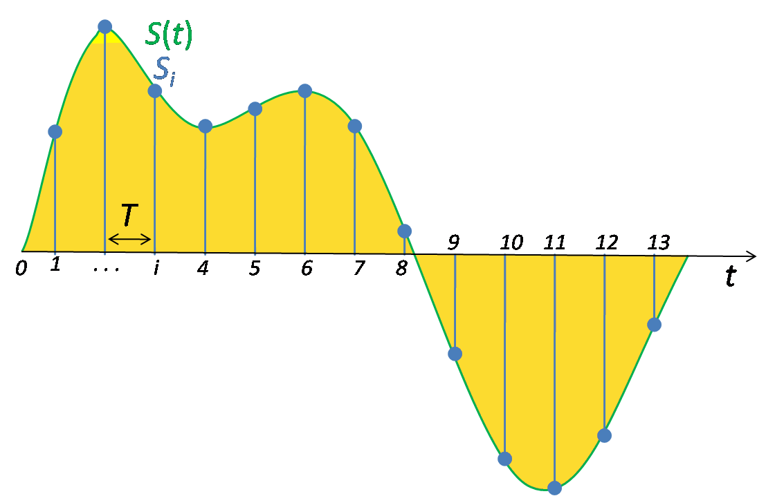
For functions that vary with time, let s(t) be a continuous function (or “signal”) to be sampled, and let sampling be performed by measuring the value of the continuous function every T seconds, which is called the sampling interval or the sampling period. Then the sampled function is given by the sequence: s(nT),   for integer values of n.

The sampling frequency or sampling rate, f_s, is the average number of samples obtained in one second (samples per second), thus f_s = 1/T.

Reconstructing a continuous function from samples is done by interpolation algorithms. The Whittaker–Shannon interpolation formula is mathematically equivalent to an ideal lowpass filter whose input is a sequence of Dirac delta functions that are modulated (multiplied) by the sample values. When the time interval between adjacent samples is a constant (T), the sequence of delta functions is called a Dirac comb. Mathematically, the modulated Dirac comb is equivalent to the product of the comb function with s(t). That purely mathematical abstraction is sometimes referred to as impulse sampling.

Most sampled signals are not simply stored and reconstructed. But the fidelity of a theoretical reconstruction is a customary measure of the effectiveness of sampling. That fidelity is reduced when s(t) contains frequency components whose periodicity is smaller than two samples; or equivalently the ratio of cycles to samples exceeds ½ (see Aliasing). The quantity ½ cycles/sample × f_s samples/sec = f_s/2 cycles/sec (hertz) is known as the Nyquist frequency of the sampler. Therefore, s(t) is usually the output of a lowpass filter, functionally known as an anti-aliasing filter. Without an anti-aliasing filter, frequencies higher than the Nyquist frequency will influence the samples in a way that is misinterpreted by the interpolation process.

Practical considerations

In practice, the continuous signal is sampled using an analog-to-digital converter (ADC), a device with various physical limitations. This results in deviations from the theoretically perfect reconstruction, collectively referred to as distortion.

Various types of distortion can occur, including:

• Aliasing. Some amount of aliasing is inevitable because only theoretical, infinitely long, functions can have no frequency content above the Nyquist frequency. Aliasing can be made arbitrarily small by using a sufficiently large order of the anti-aliasing filter.
• Aperture error results from the fact that the sample is obtained as a time average within a sampling region, rather than just being equal to the signal value at the sampling instant . In a capacitor-based sample and hold circuit, aperture errors are introduced by multiple mechanisms. For example, the capacitor cannot instantly track the input signal and the capacitor can not instantly be isolated from the input signal.
• Jitter or deviation from the precise sample timing intervals.
• Noise, including thermal sensor noise, analog circuit noise, etc.
• Slew rate limit error, caused by the inability of the ADC input value to change sufficiently rapidly.
• Quantization as a consequence of the finite precision of words that represent the converted values.
• Error due to other non-linear effects of the mapping of input voltage to converted output value (in addition to the effects of quantization).

Although the use of oversampling can completely eliminate aperture error and aliasing by shifting them out of the pass band, this technique cannot be practically used above a few GHz, and may be prohibitively expensive at much lower frequencies. Furthermore, while oversampling can reduce quantization error and non-linearity, it cannot eliminate these entirely. Consequently, practical ADCs at audio frequencies typically do not exhibit aliasing, aperture error, and are not limited by quantization error. Instead, analog noise dominates. At RF and microwave frequencies where oversampling is impractical and filters are expensive, aperture error, quantization error and aliasing can be significant limitations.

Jitter, noise, and quantization are often analyzed by modeling them as random errors added to the sample values. Integration and zero-order hold effects can be analyzed as a form of low-pass filtering. The non-linearities of either ADC or DAC are analyzed by replacing the ideal linear function mapping with a proposed nonlinear function.

Applications

Audio sampling

Digital audio uses pulse-code modulation and digital signals for sound reproduction. This includes analog-to-digital conversion (ADC), digital-to-analog conversion (DAC), storage, and transmission. In effect, the system commonly referred to as digital is in fact a discrete-time, discrete-level analog of a previous electrical analog. While modern systems can be quite subtle in their methods, the primary usefulness of a digital system is the ability to store, retrieve and transmit signals without any loss of quality.

Sampling rate

A commonly seen unit of sampling rate is Hz, which stands for Hertz and means “samples per second”. As an example, 48 kHz is 48,000 samples per second.

When it is necessary to capture audio covering the entire 20–20,000 Hz range of human hearing, such as when recording music or many types of acoustic events, audio waveforms are typically sampled at 44.1 kHz (CD), 48 kHz, 88.2 kHz, or 96 kHz. The approximately double-rate requirement is a consequence of the Nyquist theorem. Sampling rates higher than about 50 kHz to 60 kHz cannot supply more usable information for human listeners. Early professional audio equipment manufacturers chose sampling rates in the region of 40 to 50 kHz for this reason.

There has been an industry trend towards sampling rates well beyond the basic requirements: such as 96 kHz and even 192 kHz Even though ultrasonic frequencies are inaudible to humans, recording and mixing at higher sampling rates is effective in eliminating the distortion that can be caused by foldback aliasing. Conversely, ultrasonic sounds may interact with and modulate the audible part of the frequency spectrum (intermodulation distortion), degrading the fidelity. One advantage of higher sampling rates is that they can relax the low-pass filter design requirements for ADCs and DACs, but with modern oversampling sigma-delta converters this advantage is less important.

The Audio Engineering Society recommends 48 kHz sampling rate for most applications but gives recognition to 44.1 kHz for Compact Disc (CD) and other consumer uses, 32 kHz for transmission-related applications, and 96 kHz for higher bandwidth or relaxed anti-aliasing filtering.^[9] Both Lavry Engineering and J. Robert Stuart state that the ideal sampling rate would be about 60 kHz, but since this is not a standard frequency, recommend 88.2 or 96 kHz for recording purposes.

A more complete list of common audio sample rates is:

Bit depth

Audio is typically recorded at 8-, 16-, and 24-bit depth, which yield a theoretical maximum signal-to-quantization-noise ratio (SQNR) for a pure sine wave of, approximately, 49.93 dB, 98.09 dB and 122.17 dB. CD quality audio uses 16-bit samples. Thermal noise limits the true number of bits that can be used in quantization. Few analog systems have signal to noise ratios (SNR) exceeding 120 dB. However, digital signal processing operations can have very high dynamic range, consequently it is common to perform mixing and mastering operations at 32-bit precision and then convert to 16- or 24-bit for distribution.

Speech sampling

Speech signals, i.e., signals intended to carry only human speech, can usually be sampled at a much lower rate. For most phonemes, almost all of the energy is contained in the 100 Hz–4 kHz range, allowing a sampling rate of 8 kHz. This is the sampling rate used by nearly all telephony systems, which use the G.711 sampling and quantization specifications.

Video sampling

Standard-definition television (SDTV) uses either 720 by 480 pixels (US NTSC 525-line) or 704 by 576 pixels (UK PAL 625-line) for the visible picture area.

High-definition television (HDTV) uses 720p (progressive), 1080i (interlaced), and 1080p (progressive, also known as Full-HD).

In digital video, the temporal sampling rate is defined the frame rate – or rather the field rate – rather than the notional pixel clock. The image sampling frequency is the repetition rate of the sensor integration period. Since the integration period may be significantly shorter than the time between repetitions, the sampling frequency can be different from the inverse of the sample time:

• 50 Hz – PAL video
• 60 / 1.001 Hz ~= 59.94 Hz – NTSC video

Video digital-to-analog converters operate in the megahertz range (from ~3 MHz for low quality composite video scalers in early games consoles, to 250 MHz or more for the highest-resolution VGA output).

When analog video is converted to digital video, a different sampling process occurs, this time at the pixel frequency, corresponding to a spatial sampling rate along scan lines. A common pixel sampling rate is:

• 13.5 MHz – CCIR 601, D1 video

Spatial sampling in the other direction is determined by the spacing of scan lines in the raster. The sampling rates and resolutions in both spatial directions can be measured in units of lines per picture height.

Spatial aliasing of high-frequency luma or chroma video components shows up as a moiré pattern.

3D sampling

The process of volume rendering samples a 3D grid of voxels to produce 3D renderings of sliced (tomographic) data. The 3D grid is assumed to represent a continuous region of 3D space. Volume rendering is common in medial imaging, X-ray computed tomography (CT/CAT), magnetic resonance imaging (MRI), positron emission tomography (PET) are some examples. It is also used for seismic tomography and other applications.

Undersampling

When a bandpass signal is sampled slower than its Nyquist rate, the samples are indistinguishable from samples of a low-frequency alias of the high-frequency signal. That is often done purposefully in such a way that the lowest-frequency alias satisfies the Nyquist criterion, because the bandpass signal is still uniquely represented and recoverable. Such undersampling is also known as bandpass sampling, harmonic sampling, IF sampling, and direct IF to digital conversion

Oversampling

Oversampling is used in most modern analog-to-digital converters to reduce the distortion introduced by practical digital-to-analog converters, such as a zero-order hold instead of idealizations like the Whittaker–Shannon interpolation formula

Complex sampling

Complex sampling (I/Q sampling) is the simultaneous sampling of two different, but related, waveforms, resulting in pairs of samples that are subsequently treated as complex numbers. When one waveform s ( t ) 1

  is the Hilbert transform of the other waveform s ( t ) 2

  the complex-valued function

is called an analytic signal,  whose Fourier transform is zero for all negative values of frequency. In that case, the Nyquist rate for a waveform with no frequencies ≥ B can be reduced to just B (complex samples/sec), instead of 2B (real samples/sec). More apparently, the equivalent baseband waveform

Although complex-valued samples can be obtained as described above, they are also created by manipulating samples of a real-valued waveform. For instance, the equivalent baseband waveform can be created without explicitly computing s ( t )

  by processing the product sequence

through a digital lowpass filter whose cutoff frequency is B/2. Computing only every other sample of the output sequence reduces the sample-rate commensurate with the reduced Nyquist rate. The result is half as many complex-valued samples as the original number of real samples. No information is lost, and the original s(t) waveform can be recovered, if necessary.

Signal sampling representation. The continuous signal is represented with a green colored line while the discrete samples are indicated by the blue vertical lines.

The top two graphs depict Fourier transforms of two different functions that produce the same results when sampled at a particular rate. The baseband function is sampled faster than its Nyquist rate, and the bandpass function is undersampled, effectively converting it to baseband. The lower graphs indicate how identical spectral results are created by the aliases of the sampling process.

by Dr. Jaydeep T. Vagh

Digital signal processing (DSP) is the use of digital processing, such as by computers or more specialized digital signal processors, to perform a wide variety of signal processing operations. The signals processed in this manner are a sequence of numbers that represent samples of a continuous variable in a domain such as time, space, or frequency.

Digital signal processing and analog signal processing are subfields of signal processing. DSP applications include audio and speech processing, sonar, radar and other sensor array processing, spectral density estimation, statistical signal processing, digital image processing, signal processing for telecommunications, control systems, biomedical engineering, seismology, among others.

DSP can involve linear or nonlinear operations. Nonlinear signal processing is closely related to nonlinear system identification[1] and can be implemented in the time, frequency, and spatio-temporal domains.

The application of digital computation to signal processing allows for many advantages over analog processing in many applications, such as error detection and correction in transmission as well as data compression.[2] DSP is applicable to both streaming data and static (stored) data.

Signal sampling

To digitally analyze and manipulate an analog signal, it must be digitized with an analog-to-digital converter (ADC). Sampling is usually carried out in two stages, discretization and quantization. Discretization means that the signal is divided into equal intervals of time, and each interval is represented by a single measurement of amplitude. Quantization means each amplitude measurement is approximated by a value from a finite set. Rounding real numbers to integers is an example.

The Nyquist–Shannon sampling theorem states that a signal can be exactly reconstructed from its samples if the sampling frequency is greater than twice the highest frequency component in the signal. In practice, the sampling frequency is often significantly higher than twice the Nyquist frequency.

Theoretical DSP analyses and derivations are typically performed on discrete-time signal models with no amplitude inaccuracies (quantization error), “created” by the abstract process of sampling. Numerical methods require a quantized signal, such as those produced by an ADC. The processed result might be a frequency spectrum or a set of statistics. But often it is another quantized signal that is converted back to analog form by a digital-to-analog converter (DAC).

Domains

In DSP, engineers usually study digital signals in one of the following domains: time domain (one-dimensional signals), spatial domain (multidimensional signals), frequency domain, and wavelet domains. They choose the domain in which to process a signal by making an informed assumption (or by trying different possibilities) as to which domain best represents the essential characteristics of the signal and the processing to be applied to it. A sequence of samples from a measuring device produces a temporal or spatial domain representation, whereas a discrete Fourier transform produces the frequency domain representation.

Time and space domains

The most common processing approach in the time or space domain is enhancement of the input signal through a method called filtering. Digital filtering generally consists of some linear transformation of a number of surrounding samples around the current sample of the input or output signal. There are various ways to characterize filters; for example:

• A linear filter is a linear transformation of input samples; other filters are nonlinear. Linear filters satisfy the superposition principle, i.e. if an input is a weighted linear combination of different signals, the output is a similarly weighted linear combination of the corresponding output signals.
• A causal filter uses only previous samples of the input or output signals; while a non-causal filter uses future input samples. A non-causal filter can usually be changed into a causal filter by adding a delay to it.
• A time-invariant filter has constant properties over time; other filters such as adaptive filters change in time.
• A stable filter produces an output that converges to a constant value with time, or remains bounded within a finite interval. An unstable filter can produce an output that grows without bounds, with bounded or even zero input.
• A finite impulse response (FIR) filter uses only the input signals, while an infinite impulse response (IIR) filter uses both the input signal and previous samples of the output signal. FIR filters are always stable, while IIR filters may be unstable.

A filter can be represented by a block diagram, which can then be used to derive a sample processing algorithm to implement the filter with hardware instructions. A filter may also be described as a difference equation, a collection of zeros and poles or an impulse response or step response.

The output of a linear digital filter to any given input may be calculated by convolving the input signal with the impulse response.

Frequency domain

Signals are converted from time or space domain to the frequency domain usually through use of the Fourier transform. The Fourier transform converts the time or space information to a magnitude and phase component of each frequency. With some applications, how the phase varies with frequency can be a significant consideration. Where phase is unimportant, often the Fourier transform is converted to the power spectrum, which is the magnitude of each frequency component squared.

The most common purpose for analysis of signals in the frequency domain is analysis of signal properties. The engineer can study the spectrum to determine which frequencies are present in the input signal and which are missing. Frequency domain analysis is also called spectrum- or spectral analysis.

Filtering, particularly in non-realtime work can also be achieved in the frequency domain, applying the filter and then converting back to the time domain. This can be an efficient implementation and can give essentially any filter response including excellent approximations to brickwall filters.

There are some commonly-used frequency domain transformations. For example, the cepstrum converts a signal to the frequency domain through Fourier transform, takes the logarithm, then applies another Fourier transform. This emphasizes the harmonic structure of the original spectrum.

Z-plane analysis

Digital filters come in both IIR and FIR types. Whereas FIR filters are always stable, IIR filters have feedback loops that may become unstable and oscillate. The Z-transform provides a tool for analyzing stability issues of digital IIR filters. It is analogous to the Laplace transform, which is used to design and analyze analog IIR filters.

Wavelet

In numerical analysis and functional analysis, a discrete wavelet transform (DWT) is any wavelet transform for which the wavelets are discretely sampled. As with other wavelet transforms, a key advantage it has over Fourier transforms is temporal resolution: it captures both frequency and location information.The accuracy of the joint time-frequency resolution is limited by the uncertainty principle of time-frequency.

Implementation

DSP algorithms may be run on general-purpose computers and digital signal processors. DSP algorithms are also implemented on purpose-built hardware such as application-specific integrated circuit (ASICs). Additional technologies for digital signal processing include more powerful general purpose microprocessors, field-programmable gate arrays (FPGAs), digital signal controllers (mostly for industrial applications such as motor control), and stream processors.

For systems that do not have a real-time computing requirement and the signal data (either input or output) exists in data files, processing may be done economically with a general-purpose computer. This is essentially no different from any other data processing, except DSP mathematical techniques (such as the FFT) are used, and the sampled data is usually assumed to be uniformly sampled in time or space. An example of such an application is processing digital photographs with software such as Photoshop.

When the application requirement is real-time, DSP is often implemented using specialized or dedicated processors or microprocessors, sometimes using multiple processors or multiple processing cores. These may process data using fixed-point arithmetic or floating point. For more demanding applications FPGAs may be used. For the most demanding applications or high-volume products, ASICs might be designed specifically for the application.

by Dr. Jaydeep T. Vagh

In mathematics and, in particular, mathematical dynamics, discrete time and continuous time are two alternative frameworks within which to model variables that evolve over time.

Discrete time

Discrete time views values of variables as occurring at distinct, separate “points in time”, or equivalently as being unchanged throughout each non-zero region of time (“time period”)—that is, time is viewed as a discrete variable. Thus a non-time variable jumps from one value to another as time moves from one time period to the next. This view of time corresponds to a digital clock that gives a fixed reading of 10:37 for a while, and then jumps to a new fixed reading of 10:38, etc. In this framework, each variable of interest is measured once at each time period. The number of measurements between any two time periods is finite. Measurements are typically made at sequential integer values of the variable “time”.

A discrete signal or discrete-time signal is a time series consisting of a sequence of quantities.

Unlike a continuous-time signal, a discrete-time signal is not a function of a continuous argument; however, it may have been obtained by sampling from a continuous-time signal. When a discrete-time signal is obtained by sampling a sequence at uniformly spaced times, it has an associated sampling rate.

Discrete-time signals may have several origins, but can usually be classified into one of two groups

• By acquiring values of an analog signal at constant or variable rate. This process is called sampling.
• By observing an inherently discrete-time process, such as the weekly peak value of a particular economic indicator.

Continuous time

In contrast, continuous time views variables as having a particular value for potentially only an infinitesimally short amount of time. Between any two points in time there are an infinite number of other points in time. The variable “time” ranges over the entire real number line, or depending on the context, over some subset of it such as the non-negative reals. Thus time is viewed as a continuous variable.

A continuous signal or a continuous-time signal is a varying quantity (a signal) whose domain, which is often time, is a continuum (e.g., a connected interval of the reals). That is, the function’s domain is an uncountable set. The function itself need not be continuous. To contrast, a discrete time signal has a countable domain, like the natural numbers.

A signal of continuous amplitude and time is known as a continuous-time signal or an analog signal. This (a signal) will have some value at every instant of time. The electrical signals derived in proportion with the physical quantities such as temperature, pressure, sound etc. are generally continuous signals. Other examples of continuous signals are sine wave, cosine wave, triangular wave etc.

The signal is defined over a domain, which may or may not be finite, and there is a functional mapping from the domain to the value of the signal. The continuity of the time variable, in connection with the law of density of real numbers, means that the signal value can be found at any arbitrary point in time.

A typical example of an infinite duration signal is:

A finite duration counterpart of the above signal could be:

The value of a finite (or infinite) duration signal may or may not be finite. For example,

is a finite duration signal but it takes an infinite value for t=0

In many disciplines, the convention is that a continuous signal must always have a finite value, which makes more sense in the case of physical signals.

For some purposes, infinite singularities are acceptable as long as the signal is integrable over any finite interval

Any analog signal is continuous by nature. Discrete-time signals, used in digital signal processing, can be obtained by sampling and quantization of continuous signals.

Continuous signal may also be defined over an independent variable other than time. Another very common independent variable is space and is particularly useful in image processing, where two space dimensions are used.

Relevant contexts

Discrete time is often employed when empirical measurements are involved, because normally it is only possible to measure variables sequentially. For example, while economic activity actually occurs continuously, there being no moment when the economy is totally in a pause, it is only possible to measure economic activity discretely. For this reason, published data on, for example, gross domestic product will show a sequence of quarterly values.

When one attempts to empirically explain such variables in terms of other variables and/or their own prior values, one uses time series or regression methods in which variables are indexed with a subscript indicating the time period in which the observation occurred. For example, yt might refer to the value of income observed in unspecified time period t, y3 to the value of income observed in the third time period, etc.

Moreover, when a researcher attempts to develop a theory to explain what is observed in discrete time, often the theory itself is expressed in discrete time in order to facilitate the development of a time series or regression model.

On the other hand, it is often more mathematically tractable to construct theoretical models in continuous time, and often in areas such as physics an exact description requires the use of continuous time. In a continuous time context, the value of a variable y at an unspecified point in time is denoted as y(t) or, when the meaning is clear, simply as y.

Types of equations

Discrete time

Discrete time makes use of difference equations, also known as recurrence relations. An example, known as the logistic map or logistic equation, is

in which r is a parameter in the range from 2 to 4 inclusive, and x is a variable in the range from 0 to 1 inclusive whose value in period t nonlinearly affects its value in the next period,

Another example models the adjustment of a priceP in response to non-zero excess demand for a product as

where δ is the positive speed-of-adjustment parameter which is less than or equal to 1, and where f is the excess demand function.

Continuous time

Continuous time makes use of differential equations. For example, the adjustment of a price P in response to non-zero excess demand for a product can be modeled in continuous time as

where the left side is the first derivative of the price with respect to time (that is, the rate of change of the price), λlambda is the speed-of-adjustment parameter which can be any positive finite number, and f is again the excess demand function.

Graphical depiction

A variable measured in discrete time can be plotted as a step function, in which each time period is given a region on the horizontal axis of the same length as every other time period, and the measured variable is plotted as a height that stays constant throughout the region of the time period. In this graphical technique, the graph appears as a sequence of horizontal steps. Alternatively, each time period can be viewed as a detached point in time, usually at an integer value on the horizontal axis, and the measured variable is plotted as a height above that time-axis point. In this technique, the graph appears as a set of dots.

The values of a variable measured in continuous time are plotted as a continuous function, since the domain of time is considered to be the entire real axis or at least some connected portion of it.